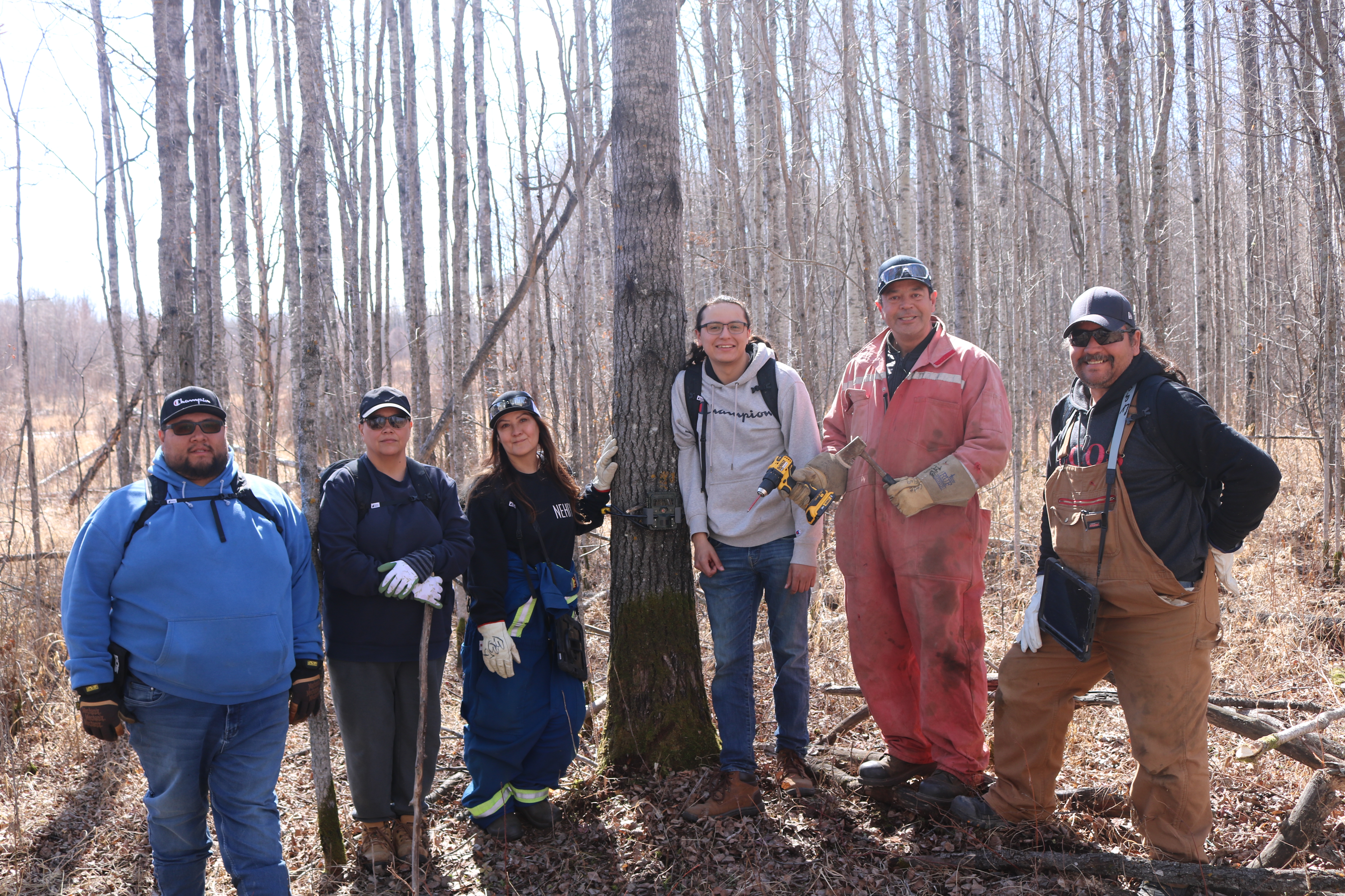
BLMS field crew deploying cameras in April 2024.
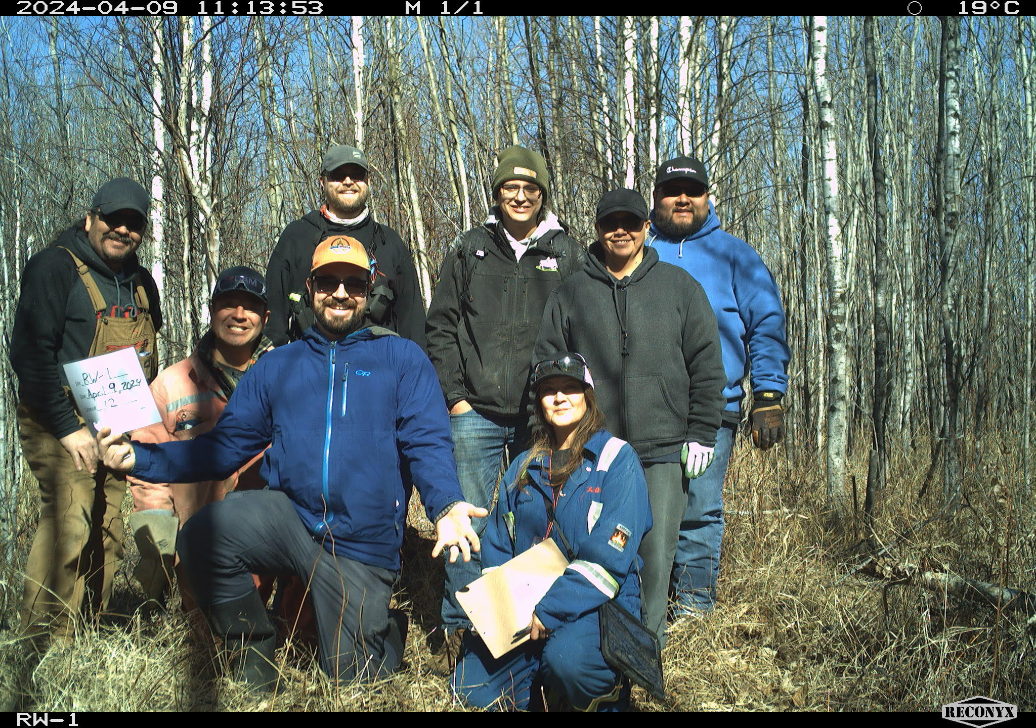
BLMS field crew with ABMI deploying cameras in April 2024.
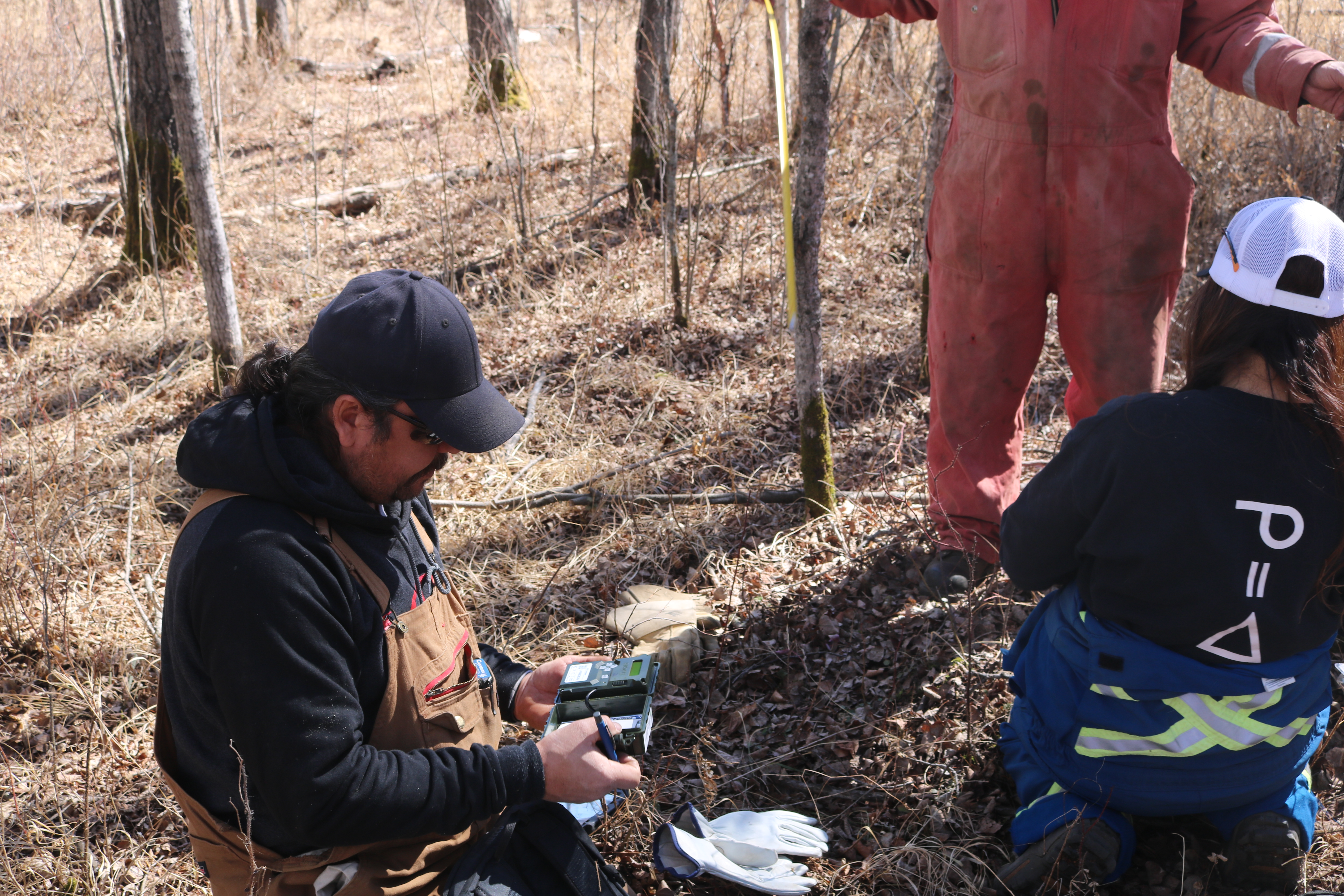
Preparing the wildlife cameras for deployment.
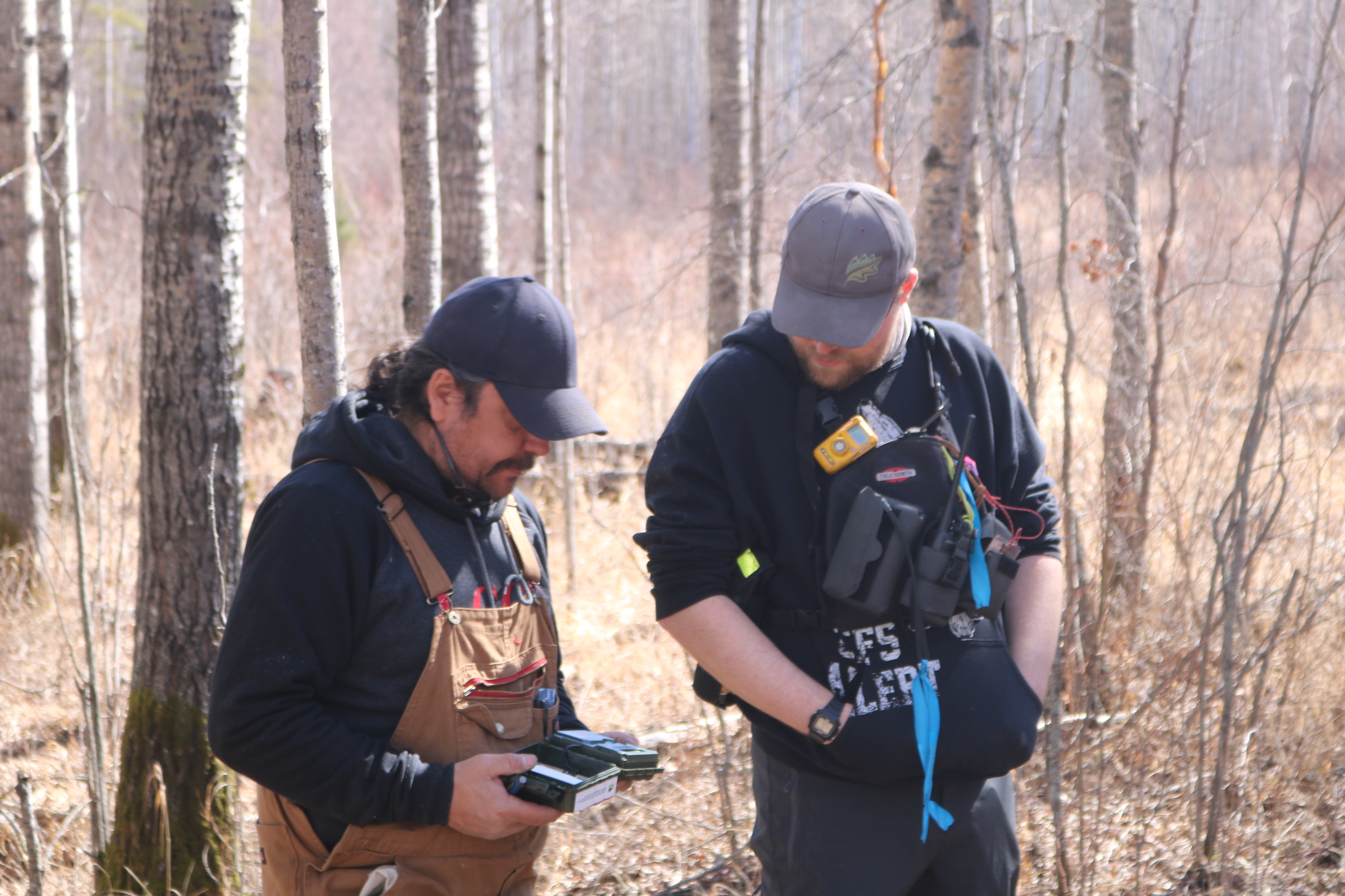
Preparing the wildlife cameras for deployment.
Results from the Cumulative Effects Wildlife Camera Project
BLMS field crew deploying cameras in April 2024.
BLMS field crew with ABMI deploying cameras in April 2024.
Preparing the wildlife cameras for deployment.
Preparing the wildlife cameras for deployment.
This report is dynamically generated, meaning its results may evolve with the addition of new data or further analyses. For the most recent updates, refer to the publication date and feel free to reach out to the authors.
The Buffalo Lake Wildlife Camera Program (BLWCP) is a community-led initiative grounded in Indigenous knowledge and stewardship values to understand how wildlife, particularly moose, supports Métis culture and way of life in northeastern Alberta. Moose are central to the Buffalo Lake Métis Settlement (BLMS) as a vital food source and cultural symbol. In response to growing concerns over oil and gas development, BLMS partnered with the Alberta Biodiversity Monitoring Institute (ABMI) to implement a camera-based wildlife monitoring program that compares two regions: one protected for wildlife conservation and one facing potential industrial development.
BLMS began this camera program in 2024 and deployed 41 cameras between April and November of 2024. Cameras were deployed in 2 grids of cameras focusing on two areas of interest to the Settlement: Rubellite West and Goose Lake. Rubellite West is to the West of the Settlement and is slated for potential oil and gas development. The Goose Lake area is within the Settlement and is a wildlife protection area. The goal of the camera program was to compare wildlife abundance between both important areas, as well as establish a baseline of wildlife abundance prior to potential development in the Rubellite West area.
The wildlife cameras were refreshed (given new SD cards and batteries) in the field by the BLMS field crew in August 2025. BLMS community members uploaded and tagged all of the camera images on the online platform WildTrax1. WildTrax is an online platform developed by the Alberta Biodiversity Monitoring Institute for users of environmental sensors such as remote cameras to provide support with processing, organizing, and sharing data. Initial results from this first year of data collected at the 40 cameras are presented here in this report.
This section is a space for BLMS staff and community members to share their major takeaways from the project so far. This could be sharing surprises from the images, camera deployment/refresh, potential to add quotes, or create videos and add them in! Highlight specific images, etc.
One idea we came up with was: One highlight of the program has been seeing how abundant the moose are in the Rubelite west camera grid area!
The following interactive map can be used to explore the locations of the cameras deployed by Buffalo Lake Métis Settlement. Satellite imagery can be switched on and off using the button in the top left of the top.
Click each camera location to see it’s name, grid, and when it was deployed and the SD cards were retrieved.
Figure 1 below displays when each camera location was deployed and when the SD cards were retrieved. Deployment took place in mid April 2024, and the majority of the cameras were serviced with new SD cards in early November 2024 after 6 months of operation. Two cameras (GLR6-SD36 and GLR12-SD14) failed earlier than the target service date, and two cameras (RW20-SD20 and RW19-SD17) were serviced at a later date.
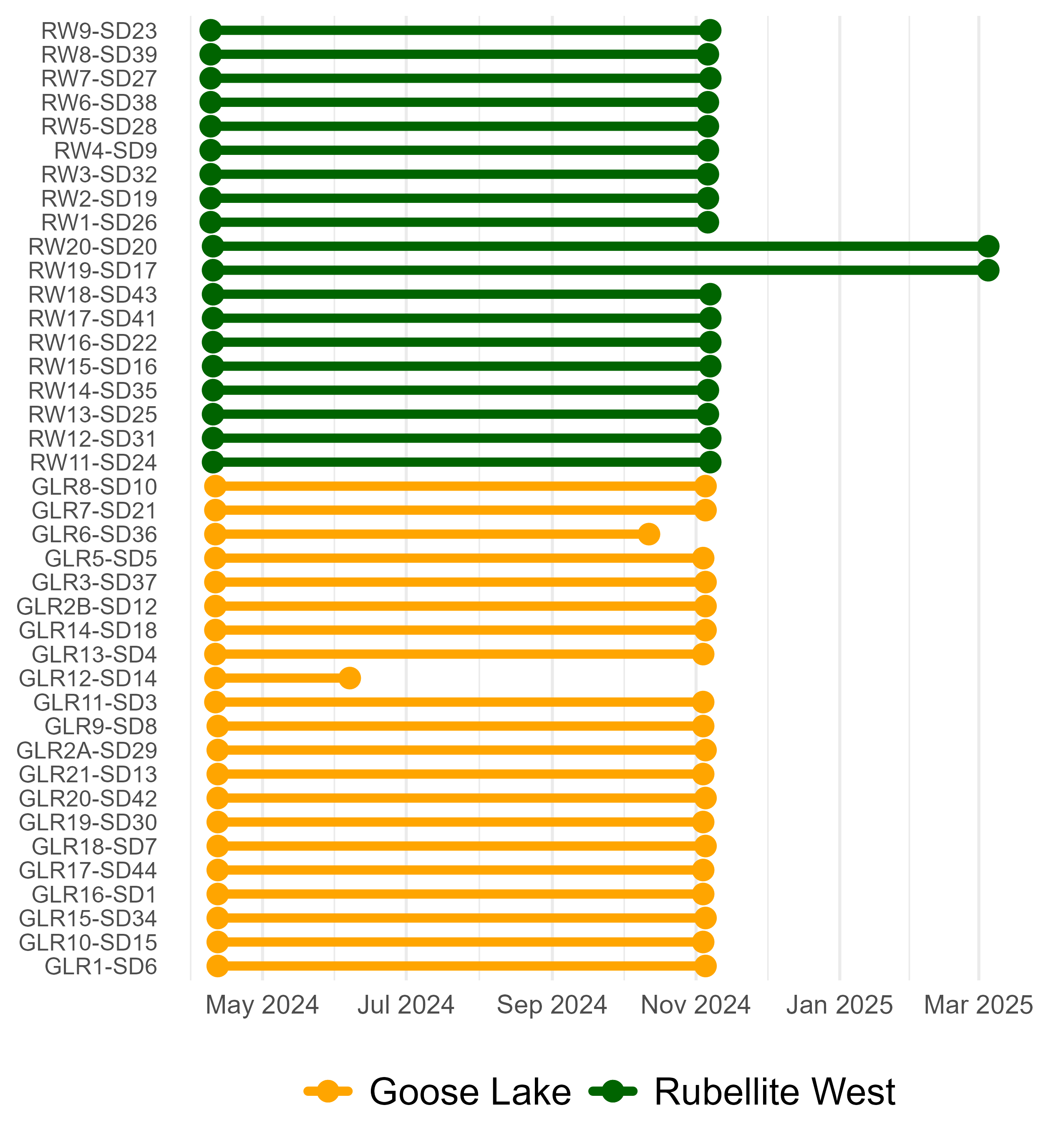
Figure 2 below displays the total number of images collected on the most common 6 species tagged in the Buffalo Lake Métis Settlement camera project. The most commonly observed species was Moose with 27745 images collected over the course of the project.
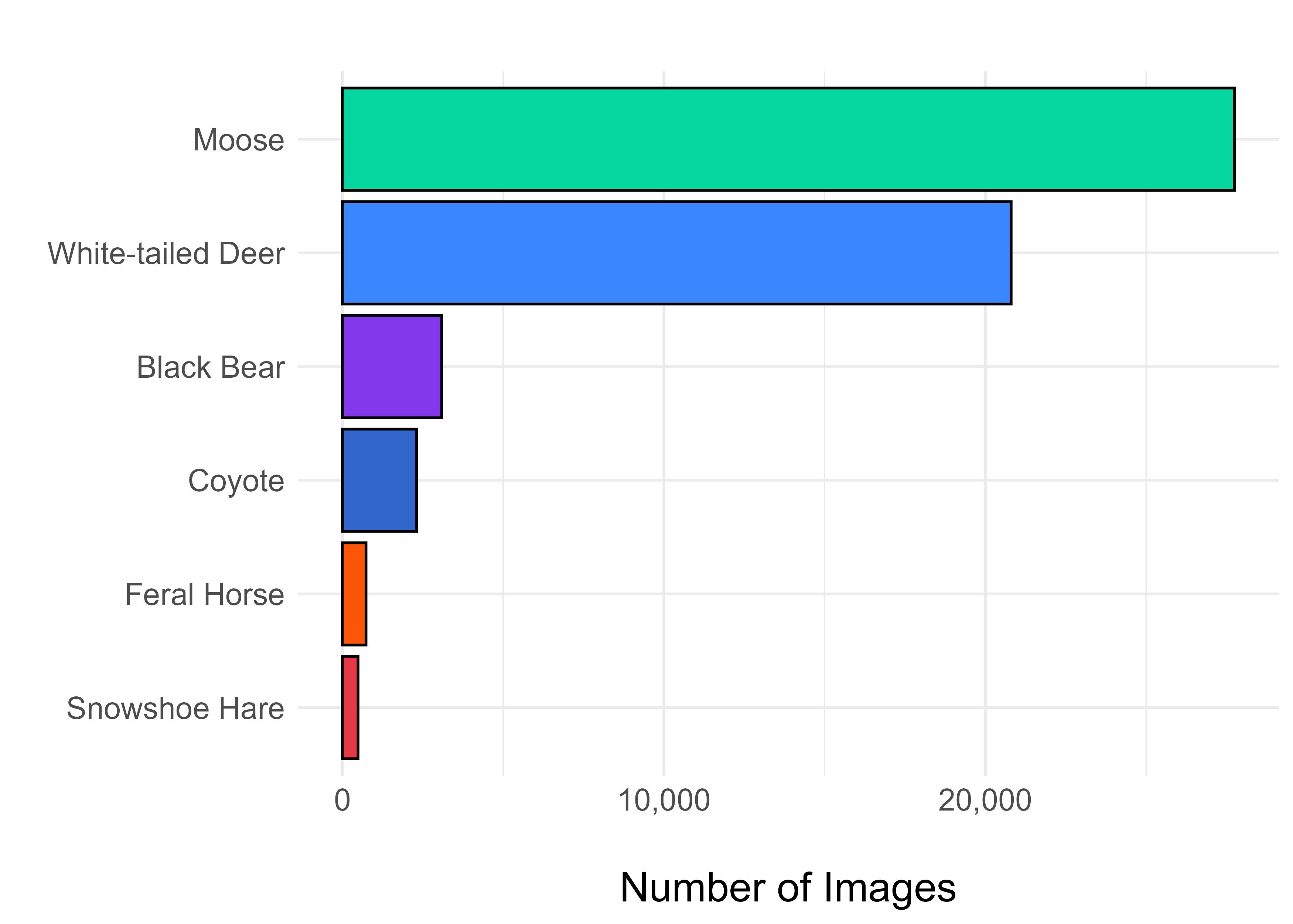
For a complete list of all the species, you can go to the project on WildTrax and click on the ‘Species’ tab of the project. Since no other species had more than 100 images collected over the course of the project and across all cameras, we will focus our analysis on the 6 species shown here (White-tailed deer, Black Bear, Moose, Coyote, Snowshoe Hare, and Feral Horse).
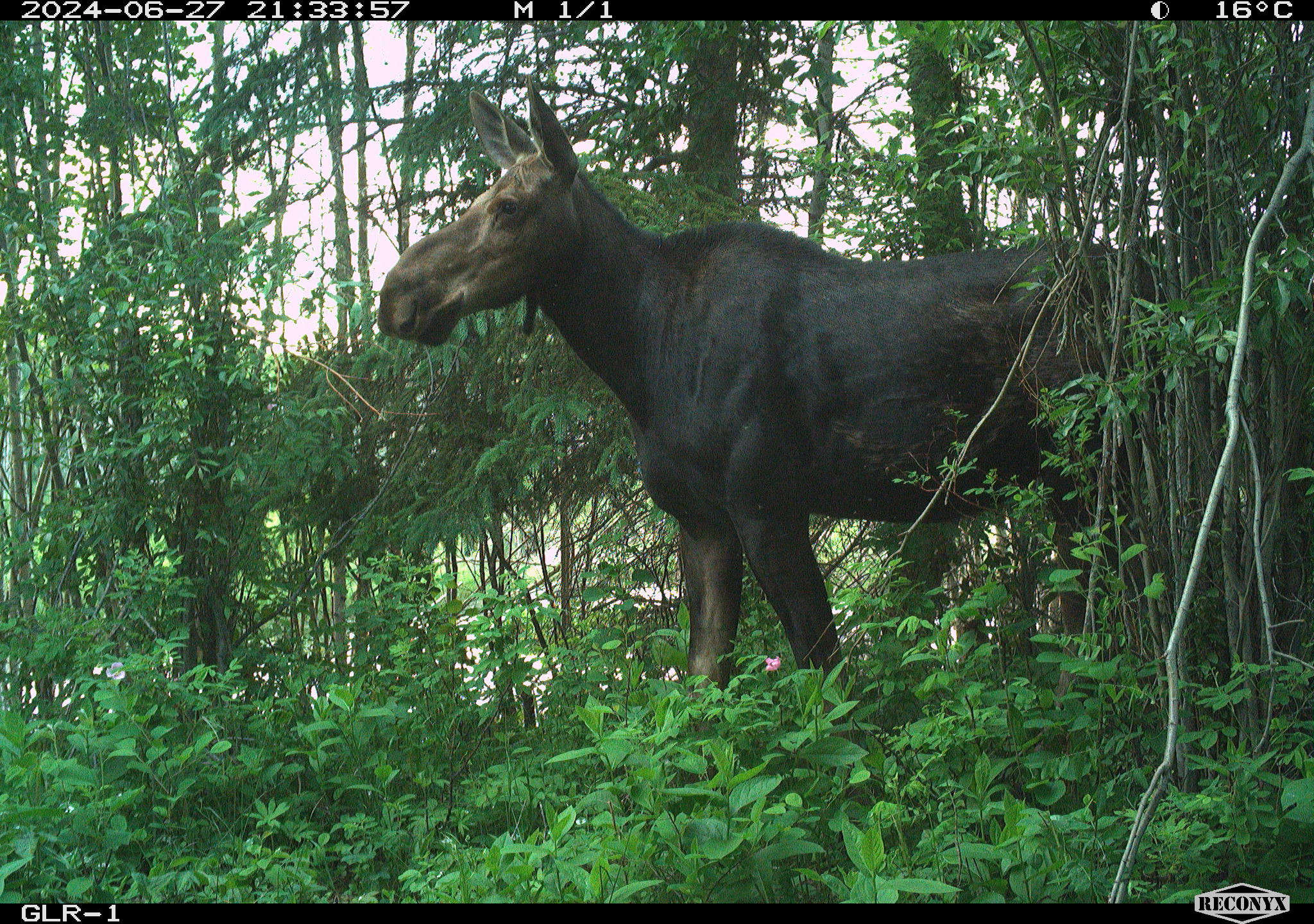
Cow moose pausing to consider her next move.
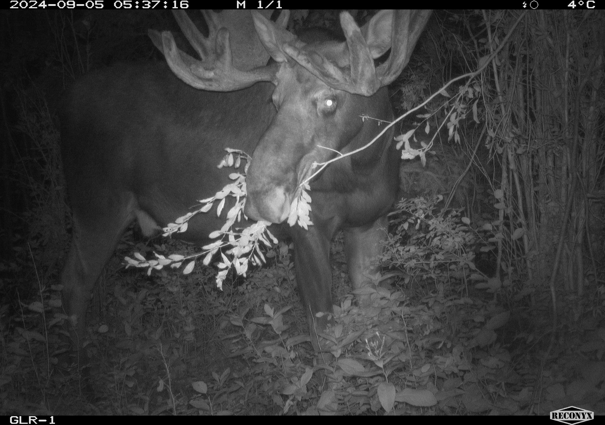
Bull moose enjoying a late night snack.
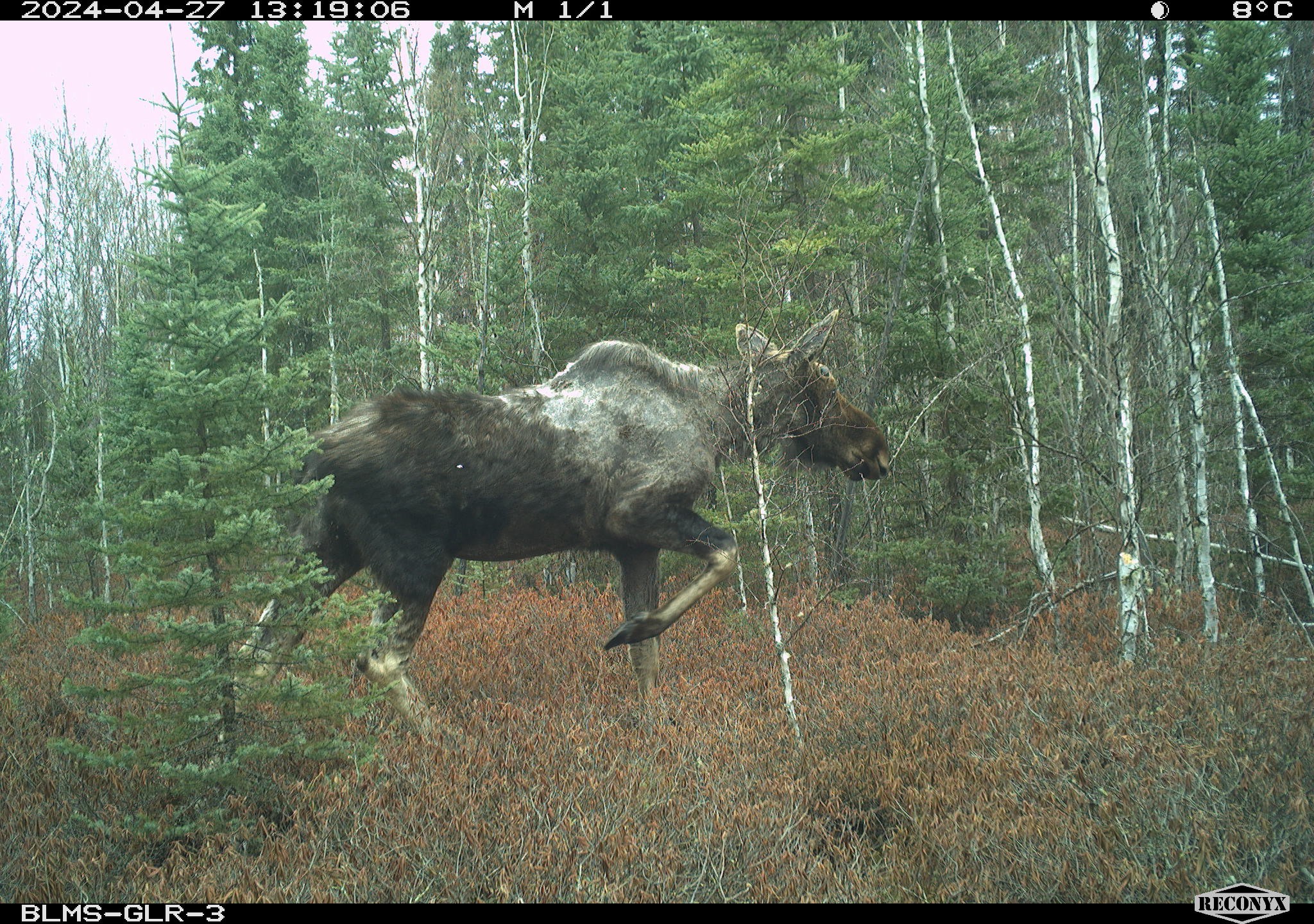
Tick infested moose with significant hair loss.
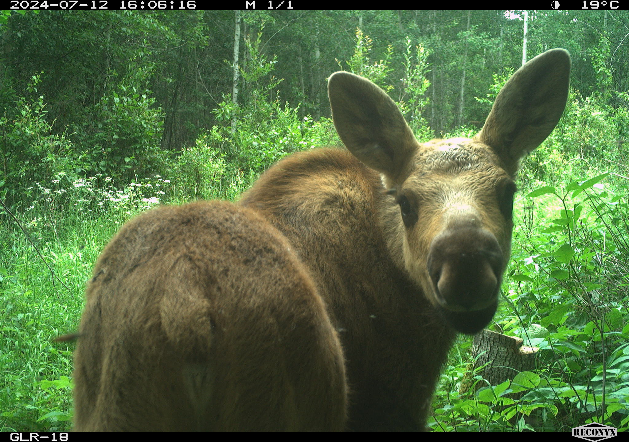
Calf posing for the camera.
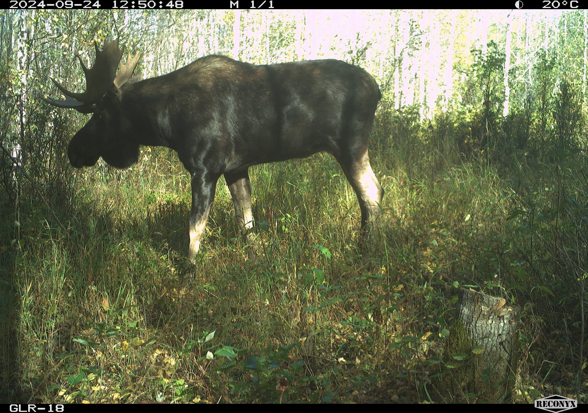
Bull moose walking along.
The number of images of each species tells us part of the picture but just because there may be more images of one species doesn’t necessarily mean there are more of them in the area, they may have just spent more time in front of the camera. With camera data, it’s important to track the number of “independent” detections for each species. You can think of an independent detection as an image or collection of images for a visit from an animal or group of animals.
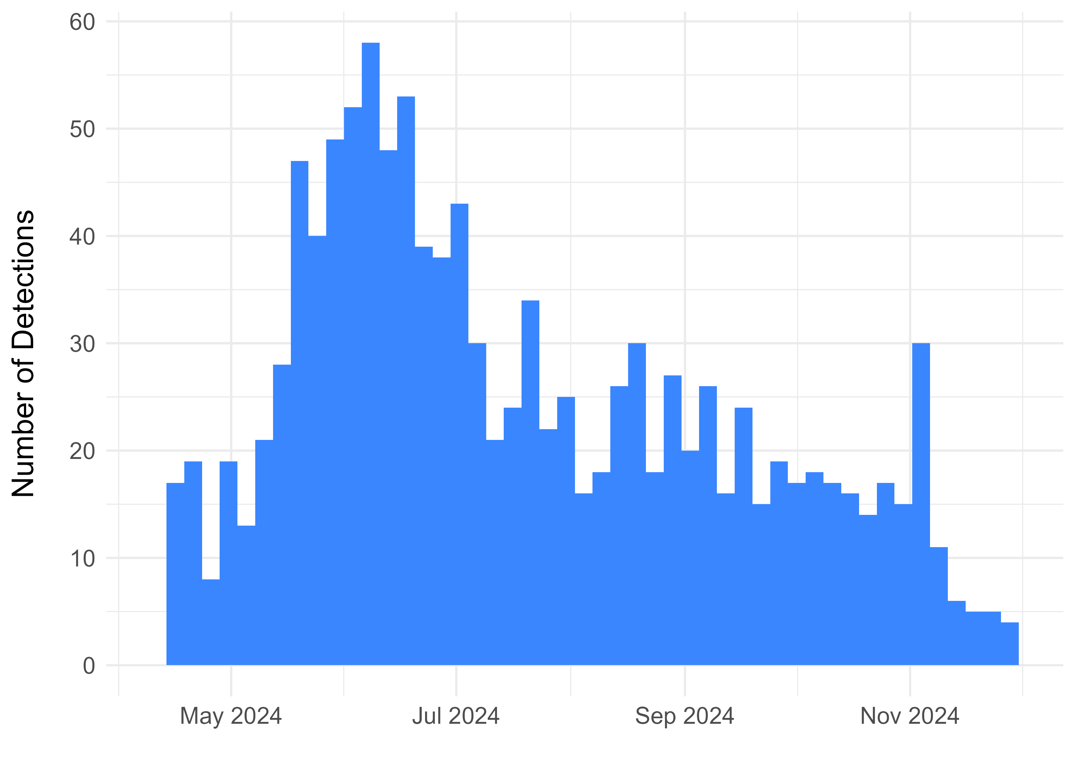
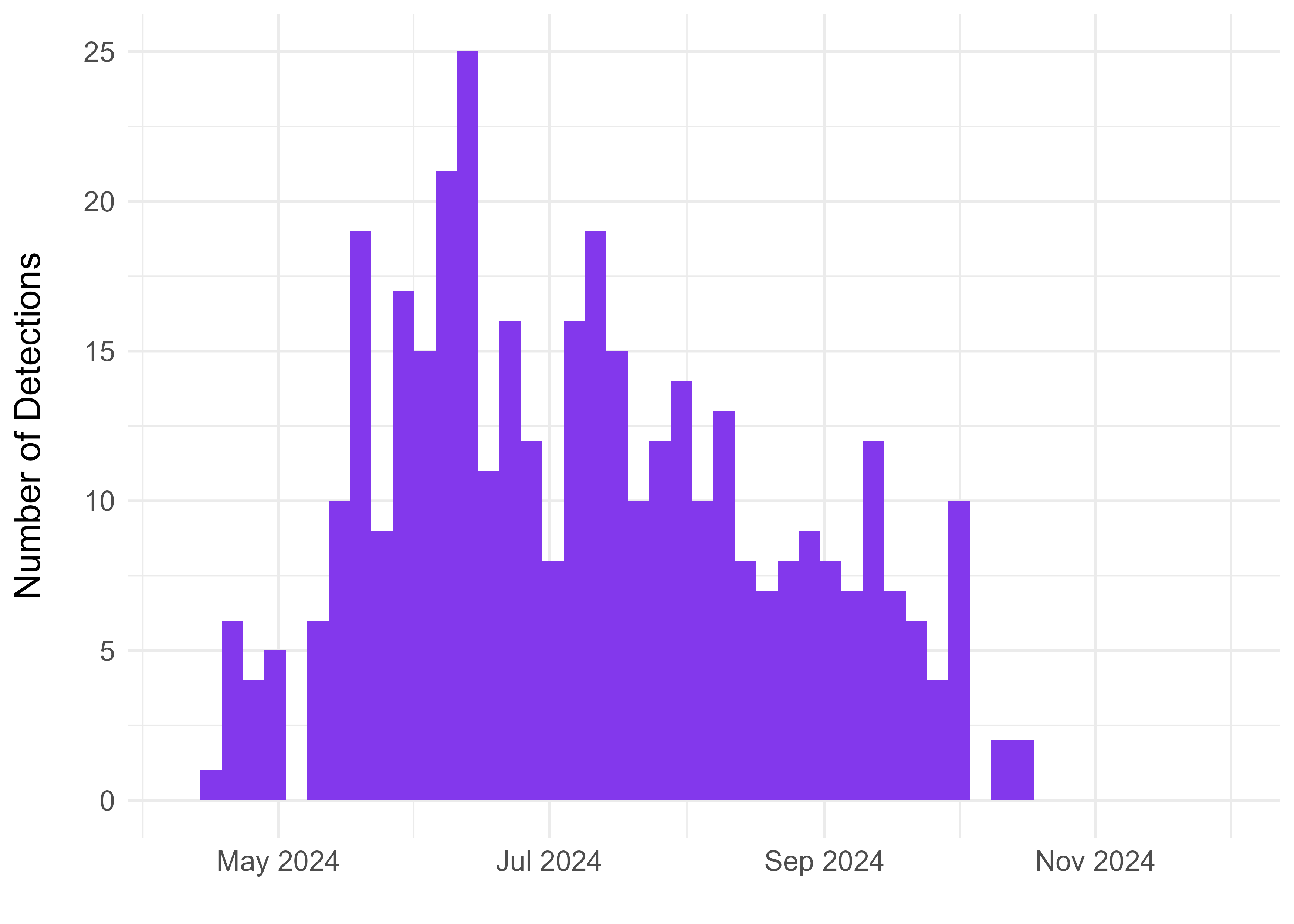
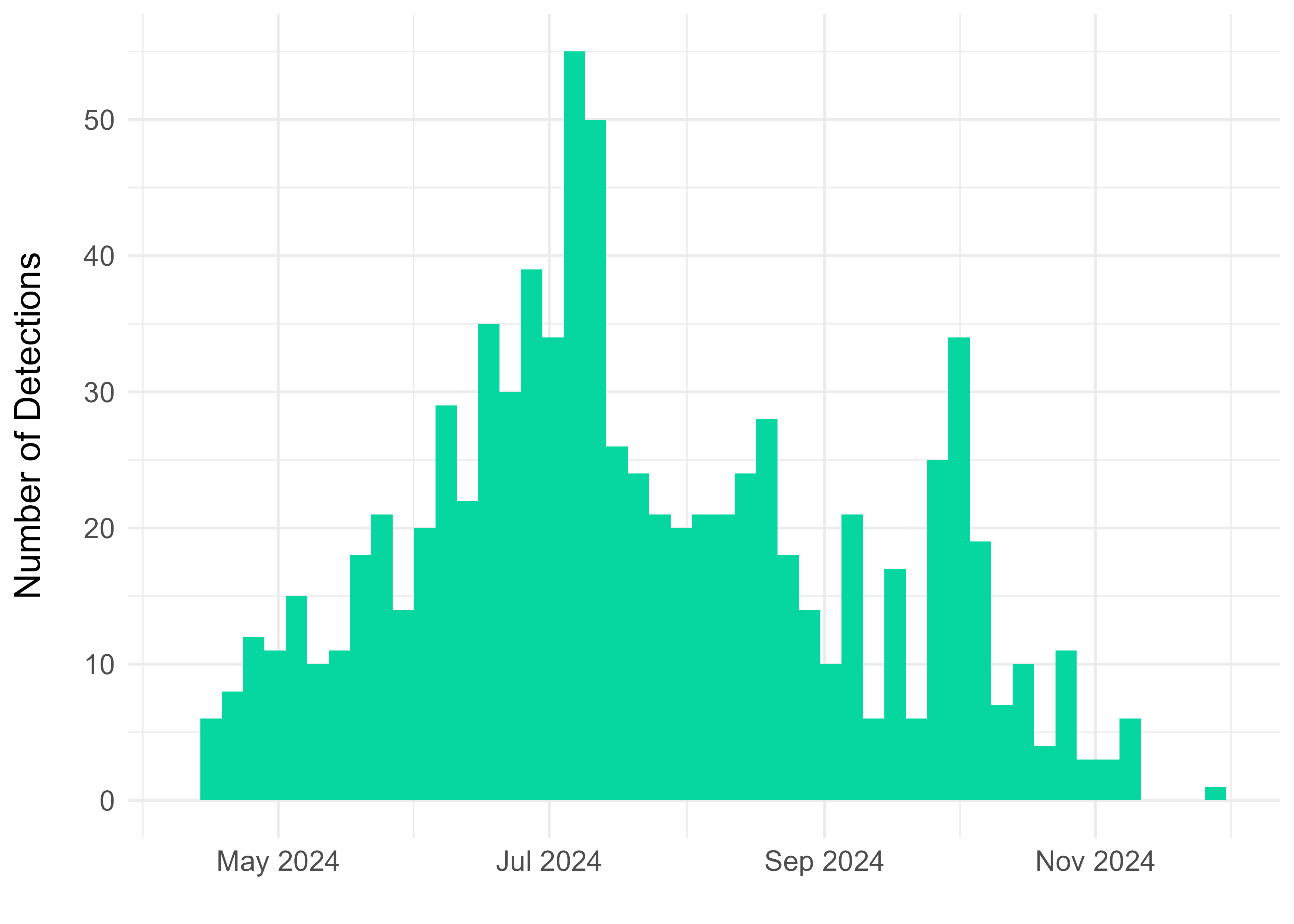
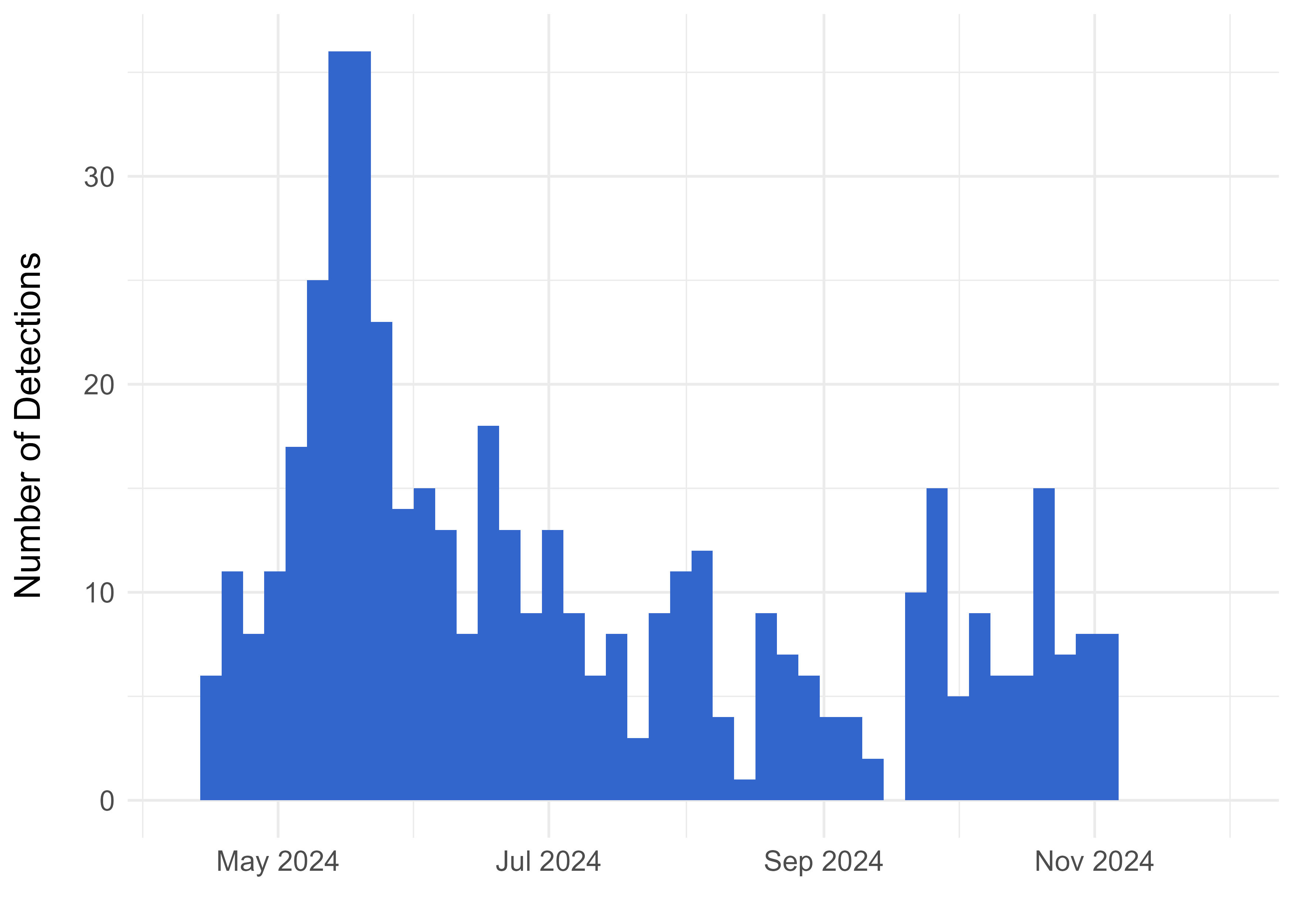
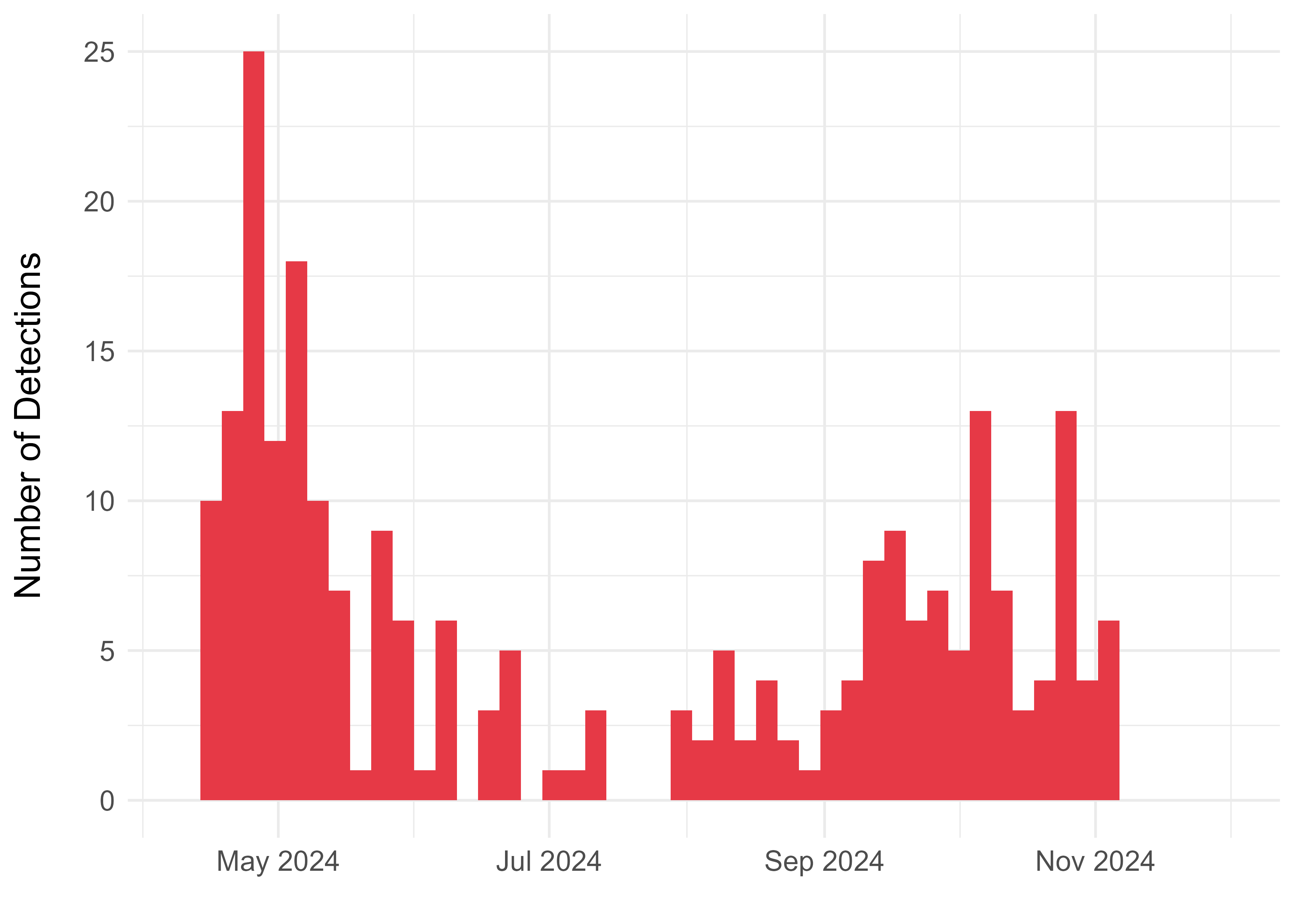
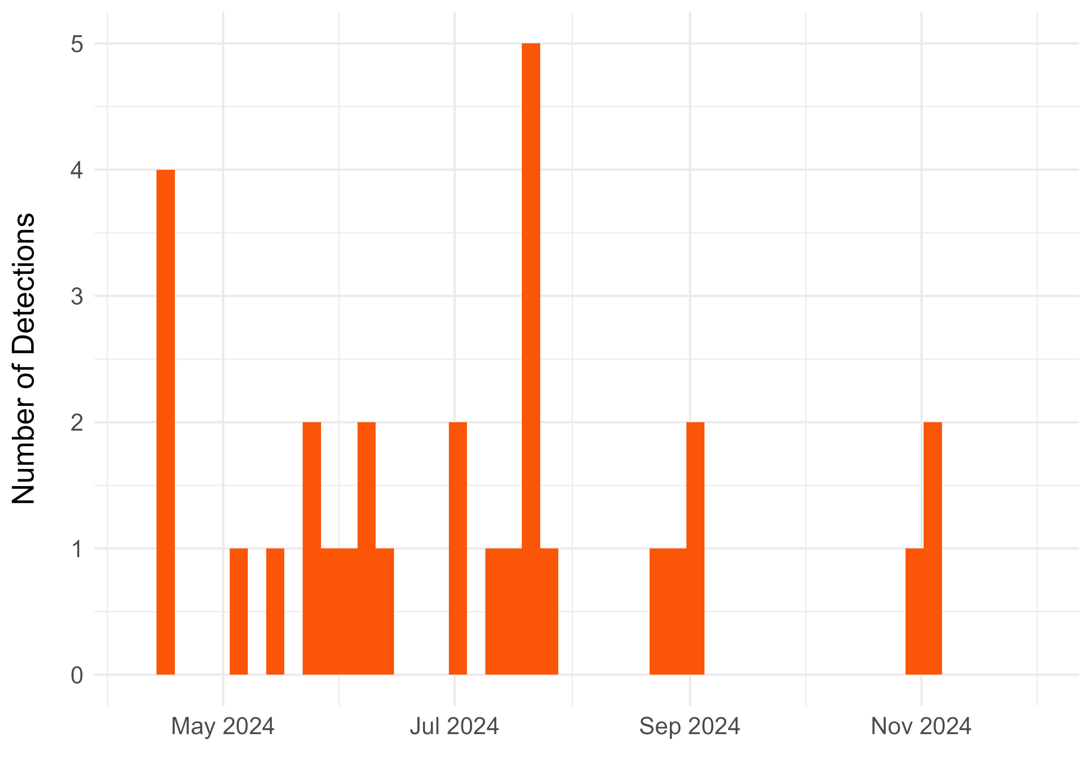
In the figure below we present the number of independent detections for each of the 6 focal species detected in the BLMS project. We use a 30 minute time interval to separate detection events; that is, images captured within 30 minutes of each other count toward a single detection and images with a gap of greater than 30 minutes between them count as multiple independent detections. Images that are captured of the same species over less than 30 minutes are assumed to be of the same individual, or group of individuals.
You can explore the figures for each species using the tabs below. The x-axis (bottom) represents the camera deployment timeline, from April 2024 to November 2024. The y-axis (left) shows the number of detections captured, from all of the cameras from the project. Note that the y-axis (left) of the plots for each species may change depending on the number of detections captured.
The table below summarises the number of images collected for each species and the number of independent detections.
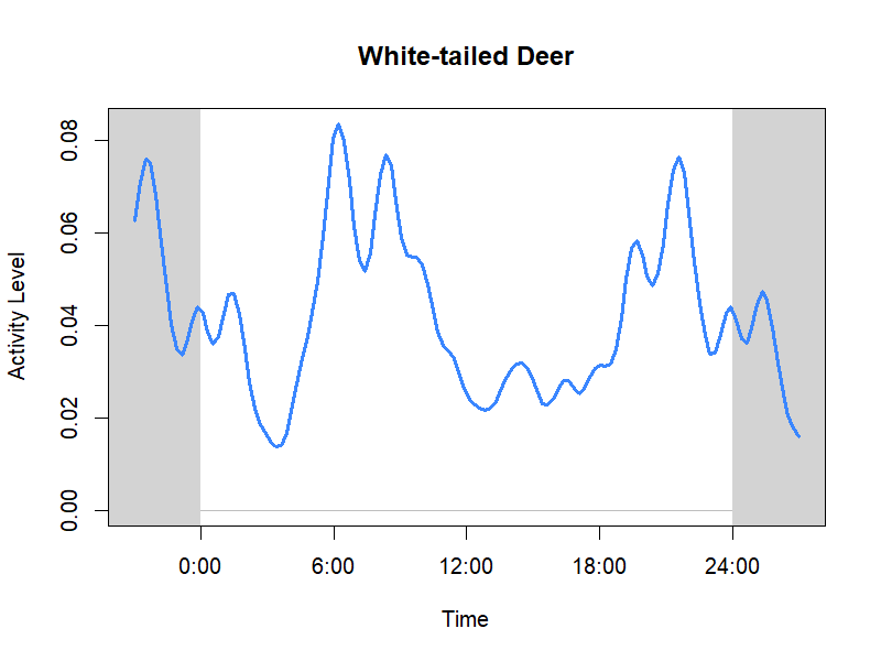
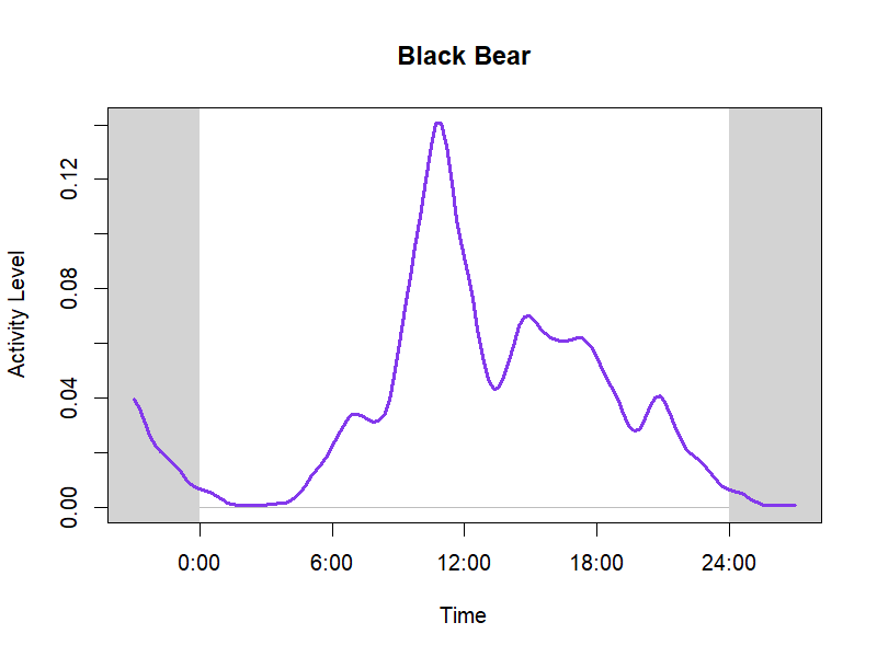
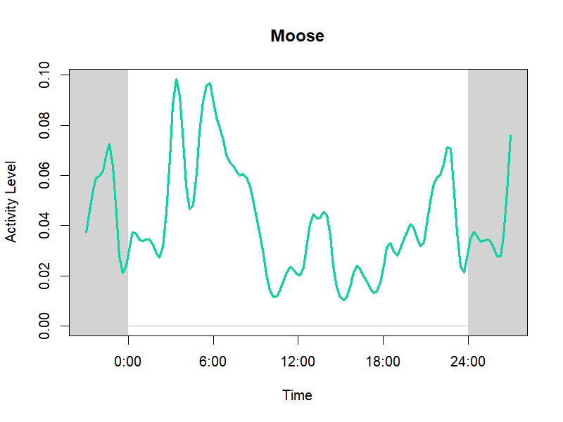
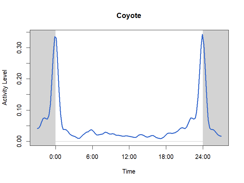
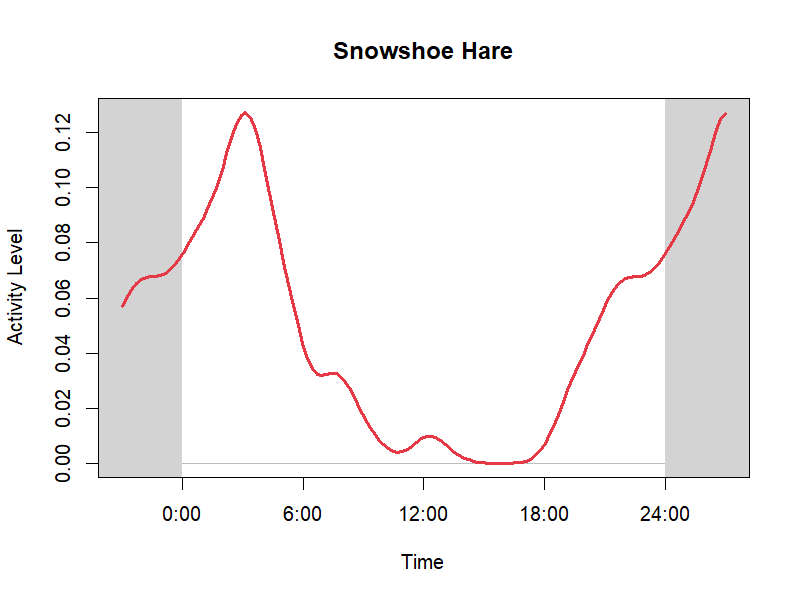
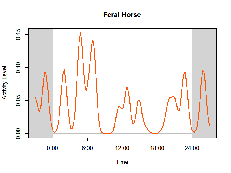
Since camera traps take photos continuously 24 hours a day they can tell us when different species are active. These analyses can give insight into competition, predation, and coexistence.
In this section we present the temporal (diel) activity patterns for each of the 6 focal species from the BLMS cameras. The x-axis (bottom) of each of the following plots represents the 24-hr daily cycle, and the line represents the relative activity level detected by the cameras. This data is pooled across all 40 cameras in the project.
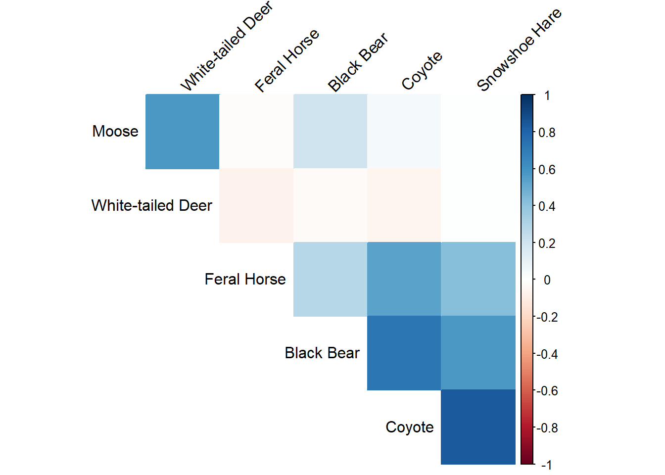
Camera trap data are being increasingly used to model multiple species communities, and we can use this data to explore the co-occurrence patterns of the species in the community.
Red (or white) boxes show species that tend to stay apart and weren’t usually seen at the same camera. For example, White-tailed Deer and Feral Horses don’t seem to share the same habitat preferences. Similarly, deer often prefer upland habitats whereas Snowshoe Hare prefer lowland areas.
We can use the number of images and counts of independent detections to estimate the density of each species at each camera. Density is the number of animals per unit area, which we express below as the number of animals per square kilometer (km2).
To estimate the density of each wildlife species at each camera, we used the Time in Front of Camera (TIFC) approach (Becker et al. (2022)). This method has previously been used to estimate densities of unmarked populations of both White-tailed Deer and Moose in the boreal region of Alberta (Laurent et al. (2021), Dickie et al. (2024)). Similar to quadrat sampling, this approach involves (for each camera) multiplying the number of animals observed by the total time they spend in front of the camera, which is then divided by the product of the area sampled by the camera and the total time the camera was operating. This calculation yields an estimate of animals per unit area (i.e., ‘density’).
The following map displays the spatial distribution in densities of the 6 focal species between the 40 cameras of the BLMS camera project. Note that cameras with no detections of a particular species (i.e., a density of ‘0’) are represented with a black circle. Smaller circles represent small densities of a species at that camera. Bigger circles indicate that the density is higher at that camera.
You can hover over each camera location to see the calculated density of each species at that deployment.
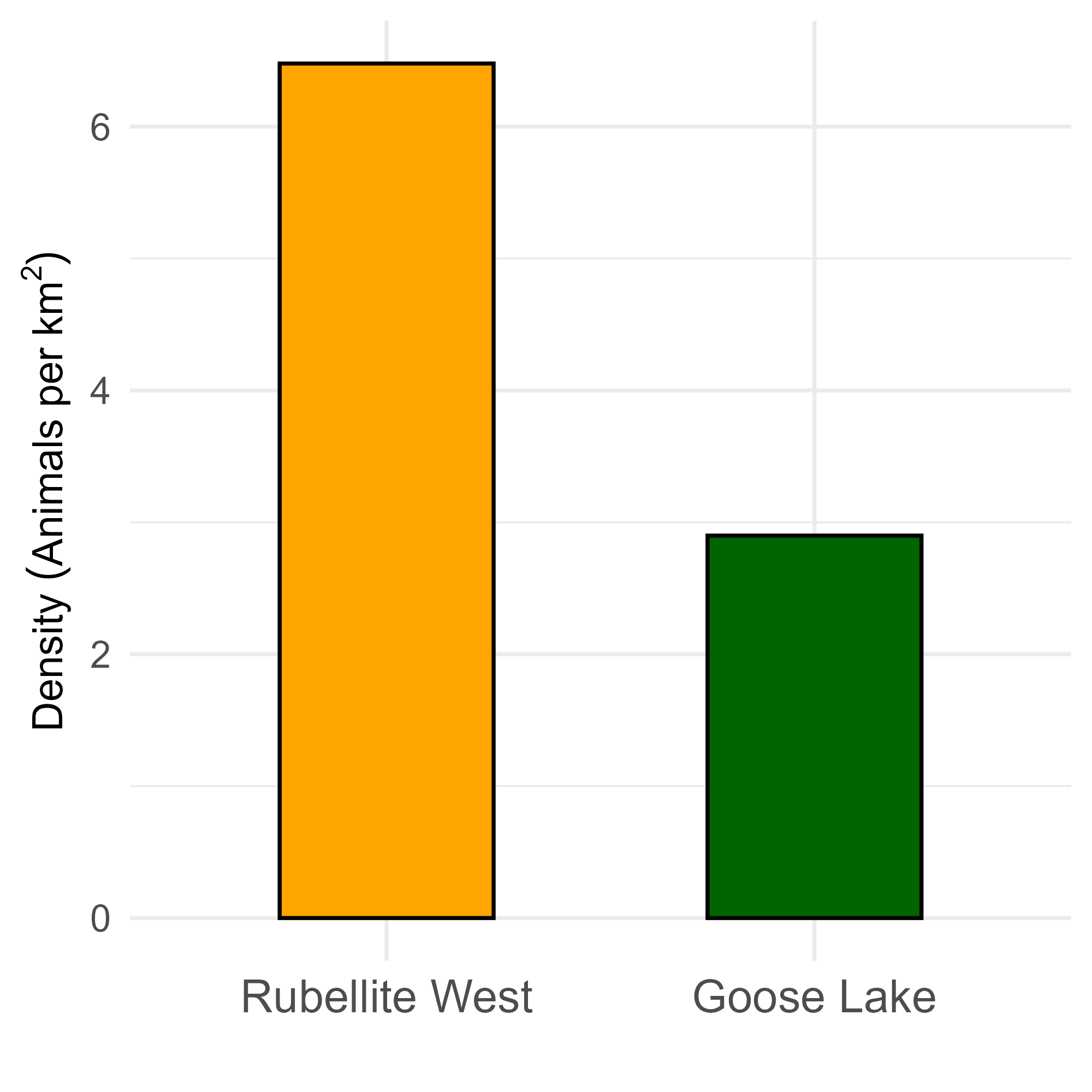
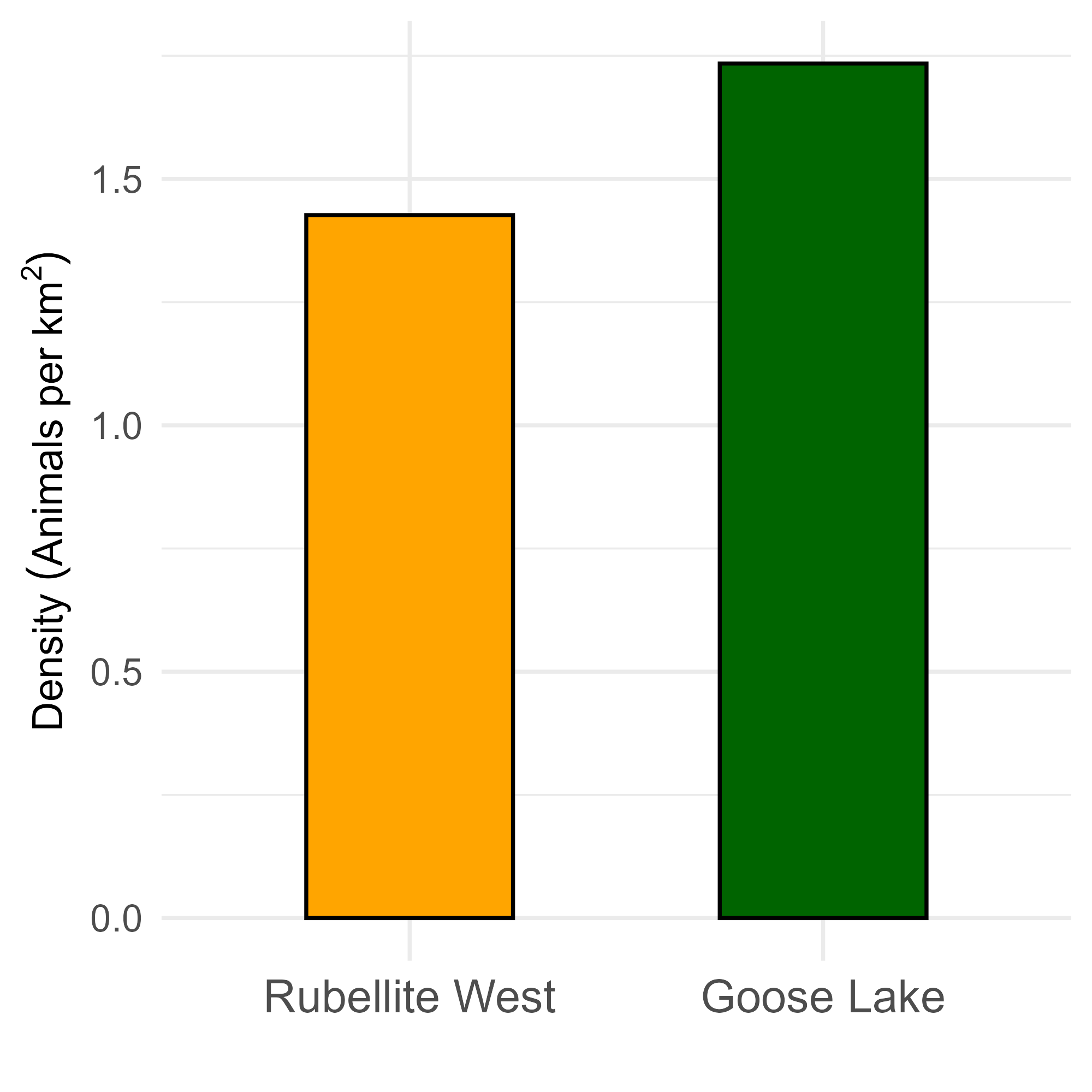
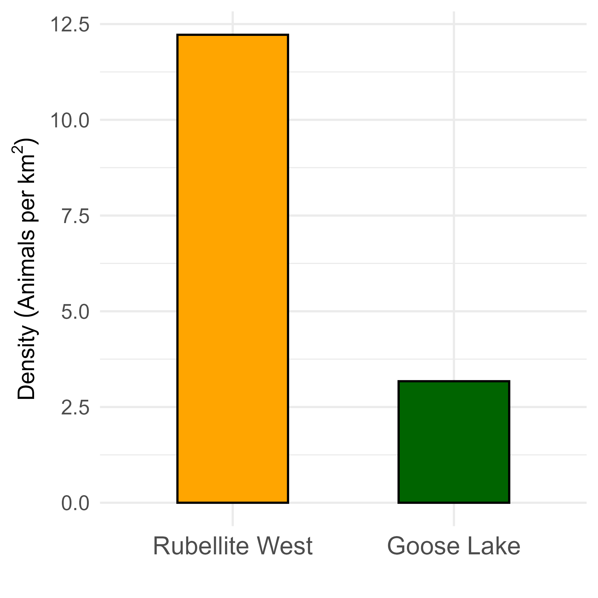
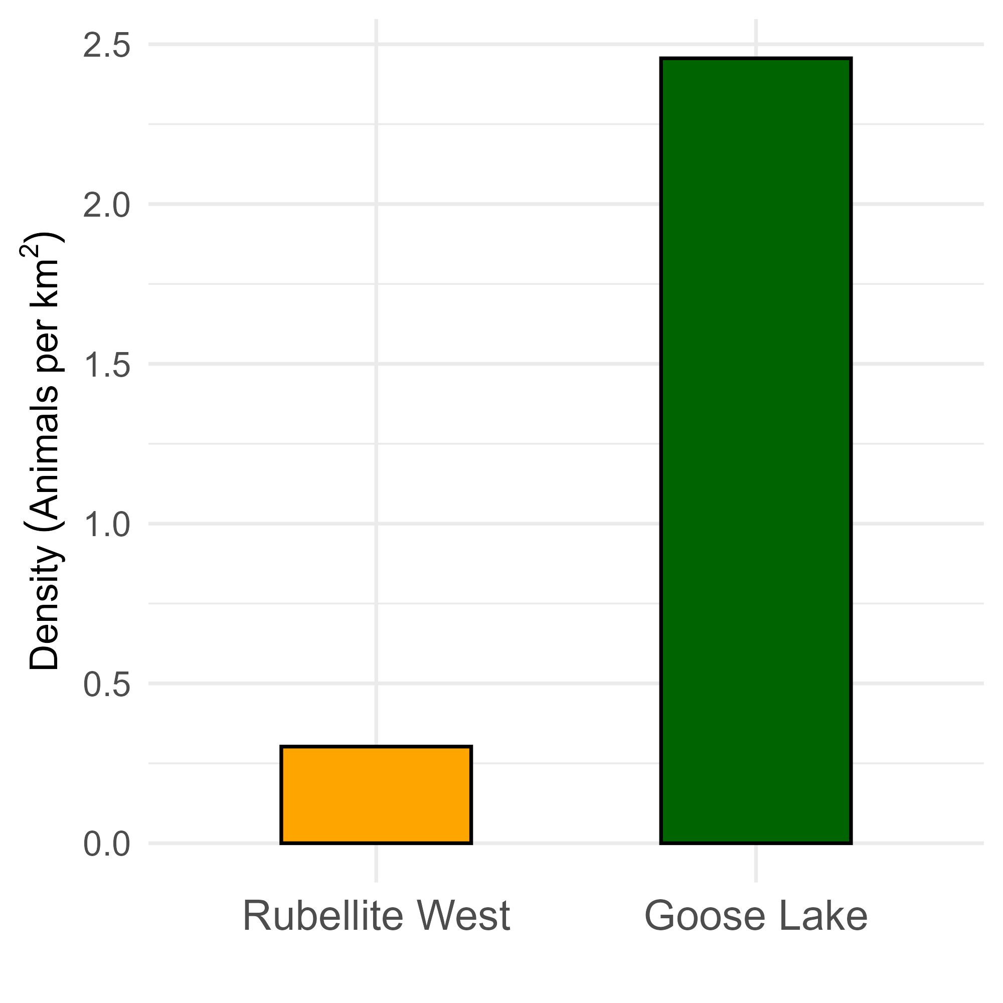
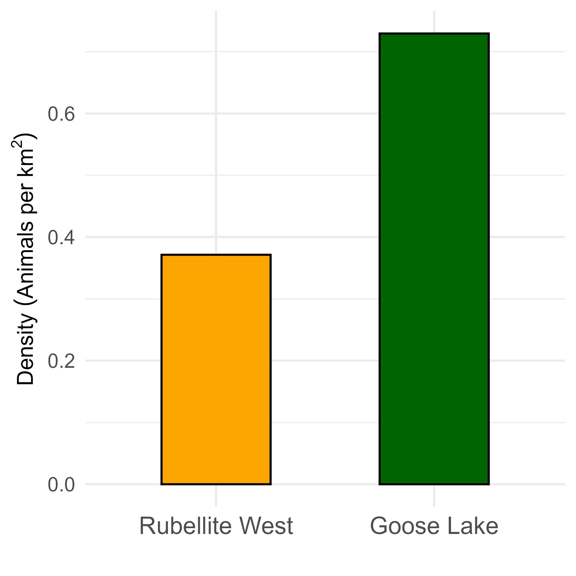
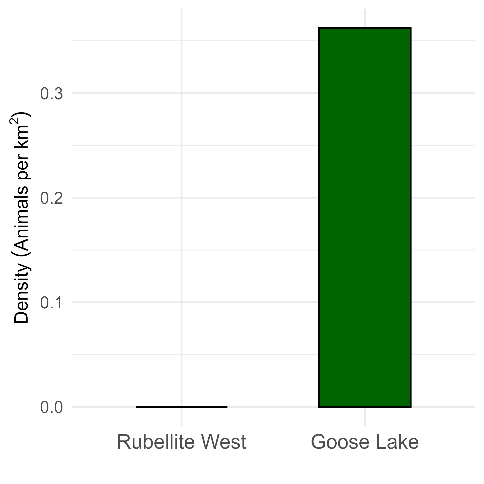
We can use the density values from the individual cameras to calculate an average density value for all the cameras within each grid (Goose Lake and Rubellite West). There were 21 cameras deployed in Goose Lake and 19 in Rubellite West. Each camera can be thought of as a sample of the larger landscape that we’re interested in (i.e., the area of the grid) so averaging together the camera values can give us an estimate of the density of the species in that area. We can then compare these average densities between grids (as well as before and after potential development) to get a sense of which area has more animals.
Figure 6 below displays the average density value for each species for both grids. Note that the y-axis (left) values differ for each species, depending on their calculated densities.
The ABMI compiles remote camera data collected in Alberta’s boreal region (including the Oil Sands Region) and uses it to develop habitat models for many species. These models incorporate species’ responses to land cover (e.g., vegetation and forest types), human disturbance, and climate variables (seasonal weather patterns).
The maps below show where the models predict each species is most likely to be found both in the BLMS settlement as well as broader area of interest. The area is divided into 1 km2 pixels, and for each pixel, the model estimates the probability of each species being there based on the habitat and disturbance present in that pixel.
Use the buttons on the top right of the map to toggle through each species’ predictions. You can also turn on Satellite Imagery and use the NONE (Blank) button to view the imagery underneath the predictions, as well as use the Camera Locations button to see where BLMS camera locations are.
(This section is available to record the direction provided by the Community to help guide the next phases of the BLMS wildlife monitoring program.)