Abundance and Sector Effects Plots

Plots the sector effects for a single or a group of species.

plot_sector(x, ...)
# S3 method for c4iraw
plot_sector(x,
    type=c("unit", "regional", "underhf"), main, ylab, subset=NULL, ...)
# S3 method for c4idf
plot_sector(x,
    type=c("unit", "regional", "underhf"), main, ylab, subset=NULL, ...)

plot_intactness(x, ...)
# S3 method for c4idf
plot_intactness(x, type=c("SI", "SI2"), col, ...)

plot_abundance(species, type, plot=TRUE, paspen=0, ...)

Arguments

x	an object of class 'c4iraw' (from `calculate_results`) or a data frame (class 'c4idf') with flattened (1-row) results per species.
species	character, species ID (see `get_all_species`).
type	type of the plot, see Details.
main	title for the plot, if single species results are displayed the default is to use the species ID.
ylab	character, optional label for the y axis.
subset	subset of sectors to be plotted, can be any suitable index.
plot	logical, if a plot is to be drawn.
paspen	numeric in [0, 1], the probability of aspen occurrence (proxy for climatic suitability for treed vegetation).
col	color.
...	other possible arguments passed to underlying functions, e.g. `ylim`, `xlab`, `ylab`, `col` (for sector colors), or `method` (one of `"kde"`, `"fft"`, or `"hist"`).

Details

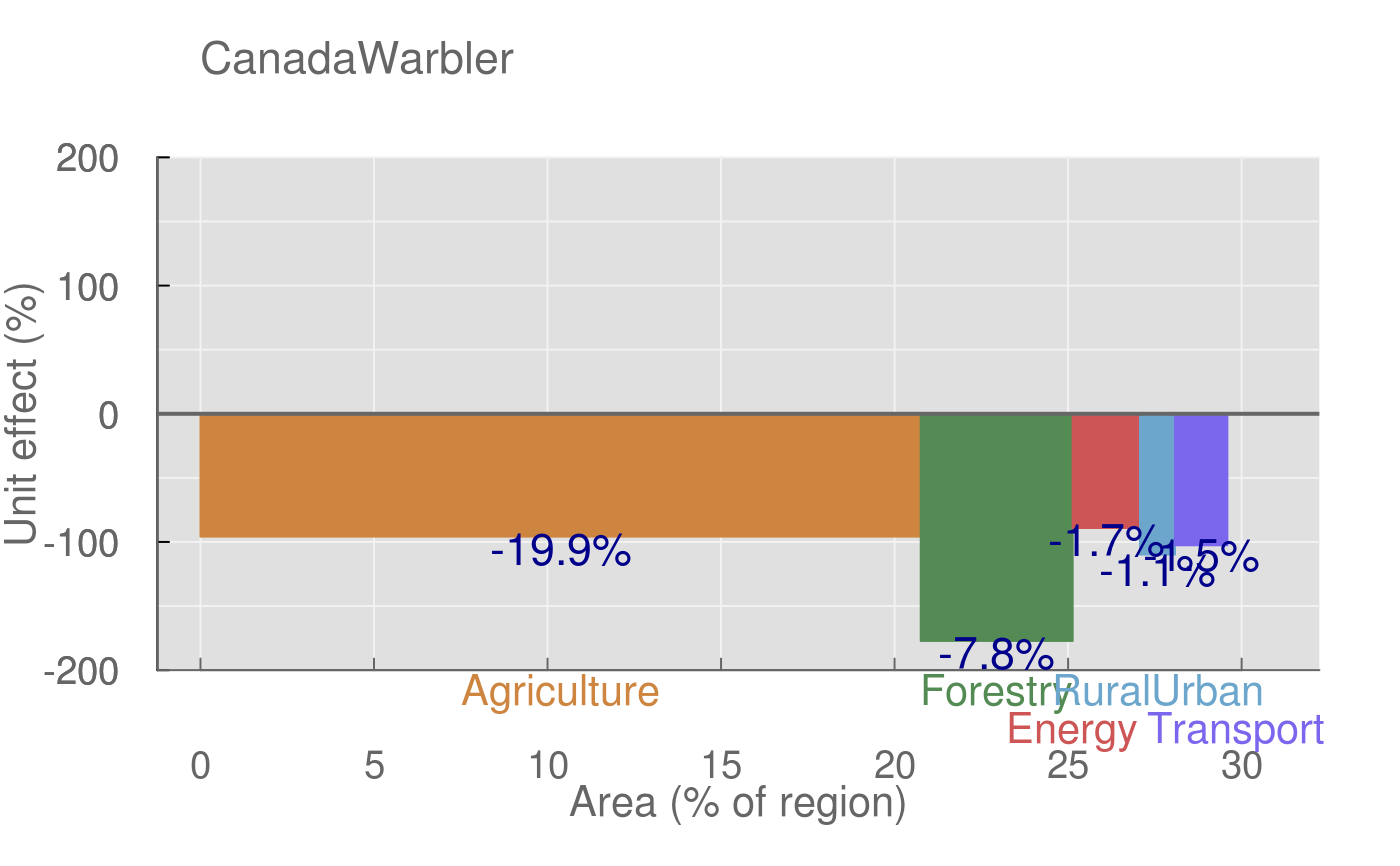
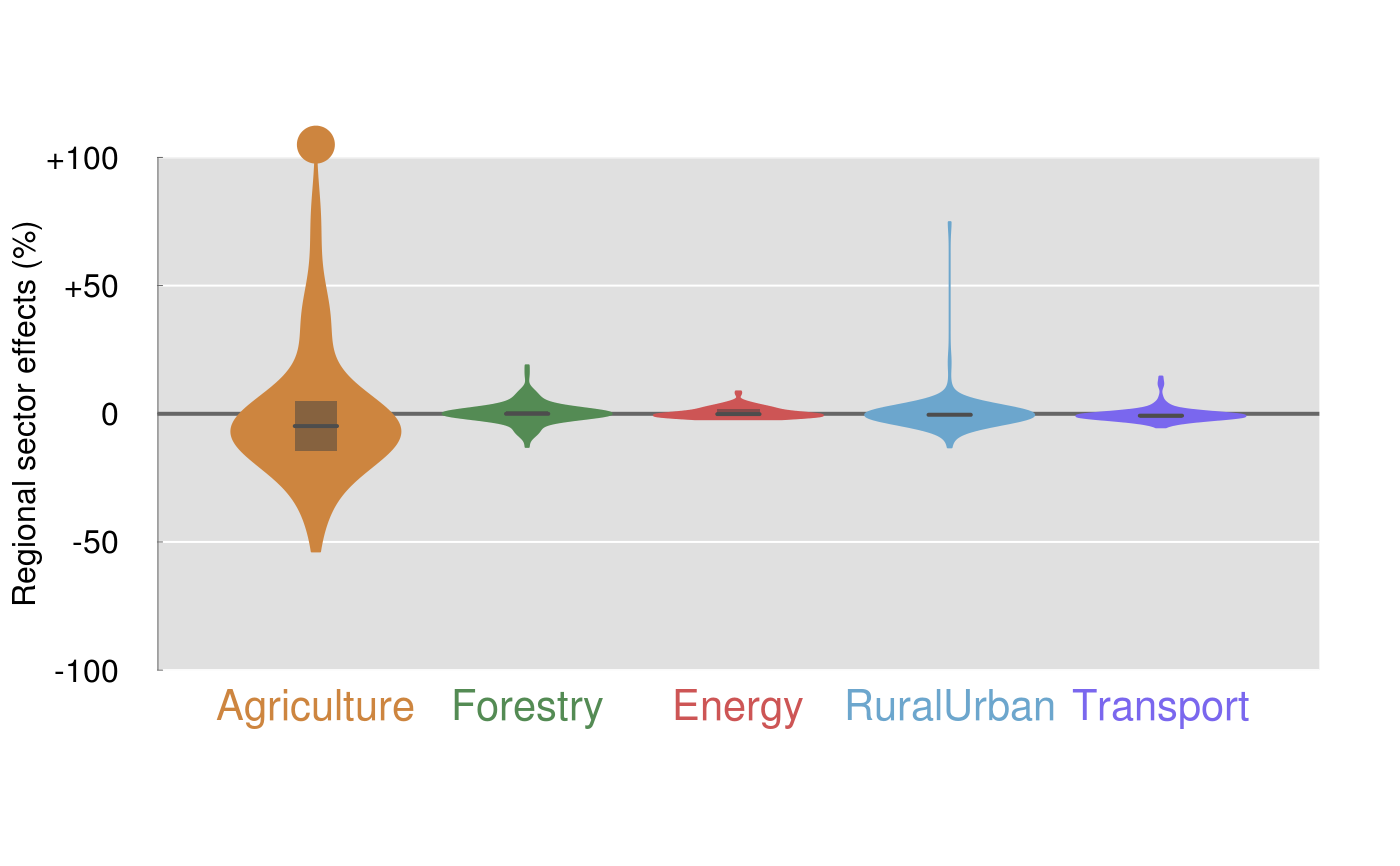
"unit" type sector effects are based on regional current and reference abundances, and the regional sector effects are standardized by footprint area.

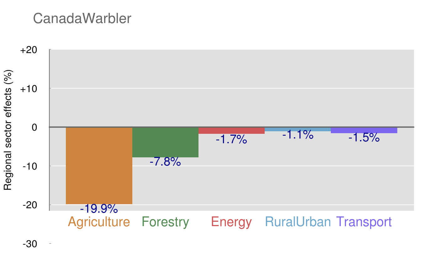
"regional" sector effects includes native and disturbed habitats when comparing regional abundance under current and reference conditions.

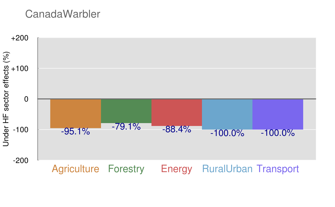
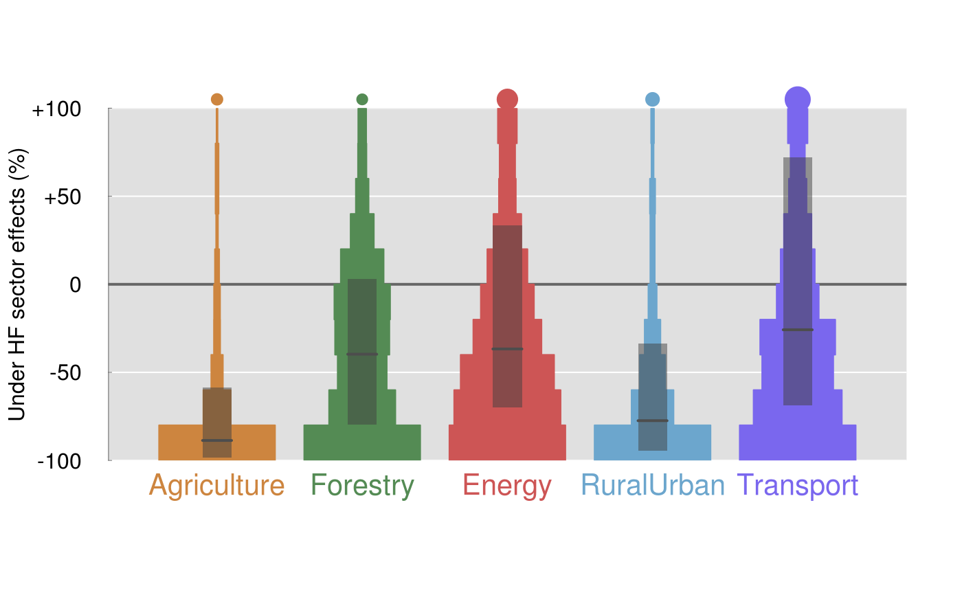
"underhf" (under human footprint) type sector effects consider only the abundance that us 'under the footprint', meaning that the current designation is disturbed.

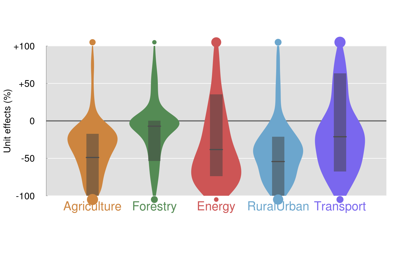
The single species sector effect plots are different kinds of bar plots. The multi-species plot represents violin (carrot, vase) plots based on kernel density, fast Fourier transform, or binning (histogram).

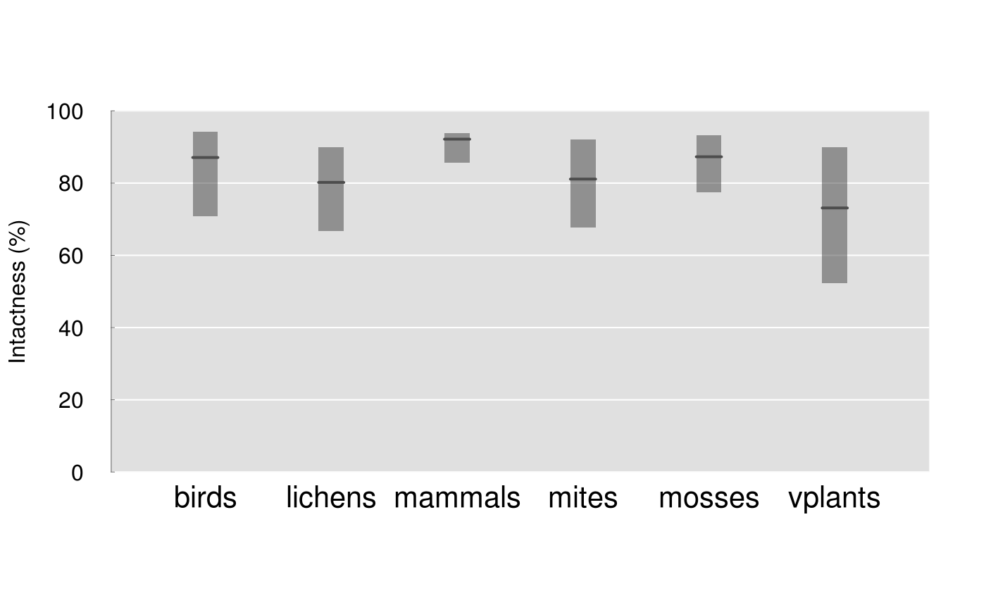
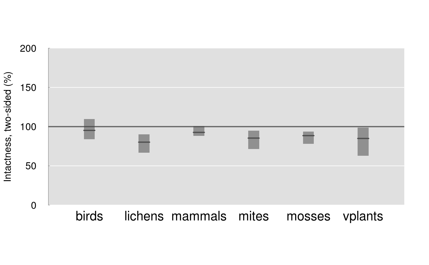
Intactness plots are either one sided (0-100%, "SI"), or two-sided (0-200%, "SI2") differentiating increased (>100%) and decreaser (<100%) species.

Abundance plots depend on the type argument: "veg_coef" type abundance plots show relative abundances across various land cover (incl. disturbance) classes, "soil_coef" shows relative abundance by soil and disturbance types. The "veg_lin" and "soil_lin" types show average relative abundances compared to 10% vegetated (soft) and non-vegetated (hard) linear disturbance.

Value

Called for the side effect of drawing a plot. Returns the plotted data invisibly.

Examples

## *res*ults from calculate_results, all province, all species
fn <- paste0("http://sc-dev.abmi.ca/reports/",
    getOption("cure4insect")$version, "/misc/raw_all.rda")
con <- url(fn)
load(con)
close(con)

plot_sector(res[["CanadaWarbler"]], "unit")
plot_sector(res[["CanadaWarbler"]], "regional")
plot_sector(res[["CanadaWarbler"]], "underhf")

z <- do.call(rbind, lapply(res, flatten))
class(z) <- c("c4idf", class(z))
plot_sector(z, "unit") # all species
plot_sector(z[1:100,], "regional") # use a subset
plot_sector(z, "underhf", method="hist") # binned version

plot_intactness(z, "SI")
plot_intactness(z, "SI2", method="hist")

if (FALSE) {
## land cover associations
load_common_data()
plot_abundance("Achillea.millefolium", "veg_coef")
plot_abundance("Achillea.millefolium", "soil_coef")
plot_abundance("Achillea.millefolium", "veg_lin")
plot_abundance("Achillea.millefolium", "soil_lin")

## R markdown file with worked examples
file.show(system.file("doc/example-species-report.Rmd", package="cure4insect"))
}

Arguments

Details

Value

See also

Examples