3 Measuring connectivity
3.1 Background
For our indicator, we chose to use the Connectivity Status Index proposed by Diebel et al. (2014). This is a biological indicator developed to identify patterns of functional connectivity within watersheds. This index provides us with the flexibility to include parameters such as habitat type, quality, and species dispersal limitations, while also incorporating variable resistance values for each barrier on the stream network. To calculate this indicator for all HUC-6 watersheds in Alberta, we required the following information:
- Provincial human footprint inventories of linear features (e.g., roads and rails) across multiple years (2010, 2014, 2016, 2018).
- Provincial stream network (ArcHydro 2).
- Locations of known dams, bridges, stream crossing inspections, and active mining leases.
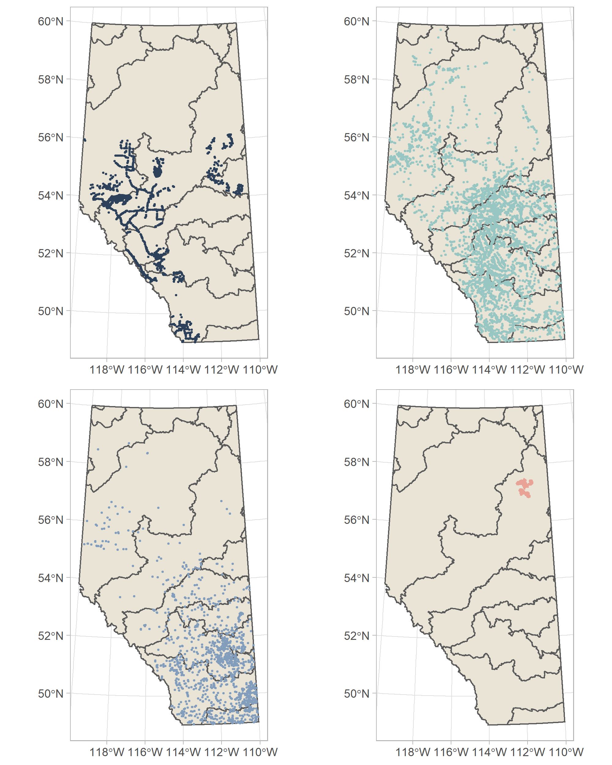
The locations of known dams, bridges, stream crossing inspections, and active mining leases.
3.2 Identifying potential barriers
Without a complete inventory of all barriers on the stream network, we need a reliable method to identify where we predict barriers to occur. We assume that all road-stream intersections will have infrastructure installed to allow for the movement of water under the road surface. In addition, all road-stream intersections are treated as culverts unless classified as a bridge (as identified by Alberta Transportation) or dam (as identified by Alberta Environment and Parks). We acknowledge there are GIS errors associated with the location of culvert surveys, bridges, and dam infrastructure. Therefore, we implemented a 50m search radius for aligning other sources of data with the predicted road-stream intersections. As dams do not necessarily occur on road-stream intersections, we used a 50m search radius to the the nearest streamline. There are also GIS errors associated with both the ArcHydro2 stream layer and human footprint inventories. These spatial errors may result in an inaccurate representation of all streams and roads, resulting in missing or artificial road-stream intersections. Though we expect improvements in the GIS layers used for this indicator, these types of spatial errors will be present in all GIS based indicators. Therefore, we recommend that ground truth surveys are performed at any location identified for management action based on the stream connectivity indicator, and associated metrics, before remediation actions are implemented.
3.3 Culvert passability model
There have been several projects focused on surveying culverts throughout Alberta in the last two decades. These projects have been wide ranging and include efforts from groups such as Parks Canada, the Alberta Conservation Association, and individual researchers who are interested in understanding how stream connectivity has been impacted across the landscape. However, these data sets are often limited in size due to the challenges associated with surveying culverts, or are restricted to priority areas in Alberta (e.g., national parks, the foothills natural region). With the creation of the Watercourse Crossing Program (WCP) and the Alberta Watercourse Crossing Inventory app (ABWCI), there has been a rapid expansion in the number of culverts being surveyed. This has been achieved due to the accessibility of the app, allowing for both professionals and citizen scientists to survey culverts, and improved collaborations between stakeholders invested in watershed management.
Using these data sets, we developed a model to predict the probability that a culvert is hanging (0 = complete hang, 1 = no hang) using the boosted-regression tree framework outlined by Januchowski-Hartley et al. (2014). We chose a subset of climatic (climate moisture index), topographic (local slope, topographic position, topographic wetness), stream (confluence bound slope, upstream distance, Strahler order), and watershed characteristics (compactness coefficient, drainage density, basin relief) as predictors of hanging culverts. These variables were chosen due to their relation to soil moisture, local and regional flow, and potential erosion rates. We created a boosted-regression tree using a learning rate of 0.001, a bag fraction rate of 0.5, and a 10-fold cross validation procedure. This model was then run through a simplification procedure to remove redundant variables. The final model used in this indicator had a cross-validation AUC score of ~0.8 and contained the following variables: climate moisture index, local slope, confluence bound slope, upstream distance, basin relief, and drainage density. We applied this model to predict the probability of hanging culverts at all road-stream intersections.
There are four situations where we purposefully mask the predictions from our hanging culvert model:
- If a culvert survey has been performed at a location, the ground truth value is used. This means that other types of barriers (e.g., garbage, sedimentation, damaged culverts etc) are incorporated into the indicator when survey data is available.
- If a road-stream intersection occurs at a known location of a bridge (as identified by Alberta Transportation), we assume there is no barrier to movement (passability = 1).
- If a road-stream intersection occurs at a known location of a dam (as identified by Alberta Environment and Parks), we assume it is a complete barrier to movement (passability = 0).
- If a road-stream intersection occurs within an active mining lease, we assume it is a complete barrier to movement (passability = 0). This is because water is required to remain within the boundary of active leases and that streams are often removed during mining activity which is not captured by our hydrology layer.
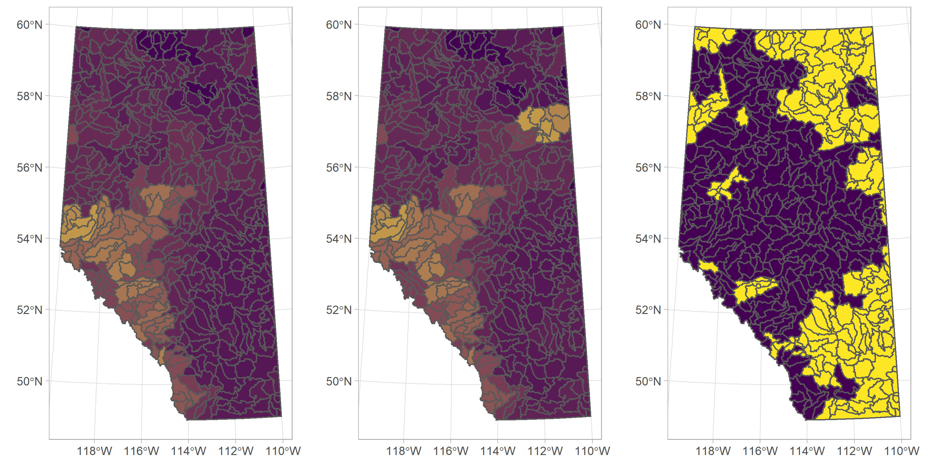
The mean passability (purple = 1, yellow = 0) of all road-stream intersections for each HUC-8 watershed. Results are visualized using only the hanging culvert model (left), by combining the hanging culvert model with the available survey, dam, minable region, and bridge information (middle), and by the directional change (purple = positive, yellow = negative) in passability between the two approaches (right).
The intent of this indicator is to focus on the impacts of anthropogenic disturbance. Therefore, we chose to focus on the dominant type of barrier on the landscape (i.e., hanging culverts) when making predictions for road-stream intersections. We acknowledge that there are other types of barriers on the landscape (e.g., waterfalls, sedimentation and garbage blockage, stream removals) and efforts will be made to incorporate them as new resources become available.
3.4 Stream Connectivity Index
For those interested in the details of the connectivity status model, we recommend you read the original paper created by Diebel et al. (2014). The main components of the index are defined as follows:
- Connectivity between segments \(i\) and \(j\) under reference condition (no artificial barriers)
\(A_{jt} = \sum_{i=1}^n(S_i \times \theta_{it} \times Q_{it} \times P_{ij}^{Nat} \times D_{ij})\)
- Connectivity between segments \(i\) and \(j\) under current conditions (artificial barriers present)
\(A_{jt}^B = \sum_{i=1}^n(S_i \times \theta_{it} \times Q_{it} \times P_{ij}^{Nat} \times P_{ij}^{Art} \times D_{ij})\)
- Inverse distance weighting function between segments \(i\) and \(j\)
\(D_{ij} = \frac{1}{1 + \frac{d_{ij}}{d_0}^2}\)
- Overall connectivity of segment \(j\)
\(C_j = \frac{\sum_{i=1, A_{jt}^B >0}^n (\frac{A_{jt}}{A_{jt}^B})}{m_j}\)
- Length-weighted average connectivity using all stream segments within a network.
\(\overline{C} = \frac{\sum_{j=1}^n (S_j \times Q_j \times C_j)}{\sum_{j=1}^n (S_j \times Q_j^\prime)}\)
Table 1. Definitions for variables included in the index. \(Q_{it}\) and \(P_{ij}^{Nat}\) are assumed to be 1 as we don’t have information on stream quality or occurrence of natural barriers at a provincial scale.
| Variable | Definition |
|---|---|
| \(S_{i}\) / \(S_{j}\) | Length of stream segments \(i\) / \(j\) |
| \(Q_{it}\) | Quality of habitat type \(t\) in stream segment \(i\) (assumed to be 1) |
| \(\theta_{it}\) | Proportion of habitat type \(t\) in stream segment \(i\) |
| \(D_{ij}\) | Inverse distance weighting function between stream segments \(i\) and \(j\) |
| \(P_{ij}^{Art}\) | Cumulative probability of passability between stream segments i and j, based on culvert passability model predictions (artificial barriers) |
| \(P_{ij}^{Nat}\) | Cumulative probability of passability between stream segments i and j, based on culvert passability model predictions (natural barriers, assumed to be 1) |
| \(d_{ij}\) | Distance between centroids of segments \(i\) and \(j\) |
| \(d_0\) | Dispersal distance constant |
| \(C_j\) | Overall connectivity of segment \(j\) |
| \(\overline{C}\) | Length-weighted average connectivity |
3.5 Dispersal Distances
The connectivity between two stream segments is weighted by the dispersal distance \(D_{0}\) of the focal species of interest. This is meant to reflect the biological differences between species as some may travel large distances throughout a network, while others are restricted to a small home range. However, the goal of this indicator was to be species agnostics. Therefore we developed an appropriate dispersal distance based on a non-biological parameter. For each stream segment, we calculated the minimum distance required to reach the highest order stream reachable within the network (HUC-6). These distances were were then averaged to represent the average distance a species must travel in order to access the main stem of the network. The final value of \(D_{0}\) used for calculating stream connectivity was 71 Km. The code base behind the indicator has the capabilities to incorporate different values of \(D_{0}\) if species specific information is desired.
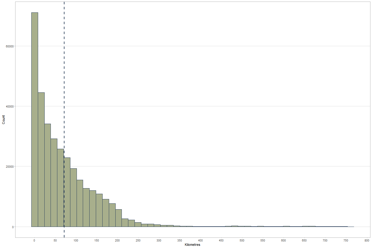
Frequency of minimum distances between stream segments and the highest order stream reachable within the stream network. The dashed line represents \(D_{0}\) which equals 71 Km.
3.6 Limitations
As with all indicators, there are limitations that can arise due to how data was collected, the spatial extent of the available data, and assumptions made in creating an index. We have identified the key limitations for this indicator that should be understood before using the results to make management decisions.
- Habitat quality can be defined using multiple measures depending on the focal species of interest (e.g., water chemistry, pollution, etc). In addition, finding habitat quality information that has a provincial spatial coverage, and is updated frequently, is challenging. Therefore, we assume habitat quality is 100% for each stream segment. The code base behind the indicator can incorporate different measurements of stream habitat quality if data is available within a focal study system.
- Stream segments can only be a single habitat type (Strahler order or Lake).
- We can only model the probability a culvert is hanging at unsampled road-stream intersections. As uptake of the ABWCI app increases, we expected to be able to model different types of barriers and increase the amount of ground truth data incorporated into the indicator.
- No information about the type of human footprint feature has been incorporated into the culvert passability model.
- Culverts are inferred based on the intersections of provided road and rails inventory and the ArcHydro2 inventory. Stream networks may change overtime, and not all roads will have culverts, so some intersections may be misrepresented.