Acoustic pre-processing • wildRtrax

The following set of functions help to pre-process and organize audio and corresponding metadata. In conjunction, these tools allow you to select recordings parameterized to a specific study design.

wt_audio_scanner() scans a directory of audio files and prepares them in a tibble with WildTrax formatted columns
wt_run_ap() allows you to generate acoustic indices and false-colour spectrograms from a wt_audio_scanner() tibble, while wt_glean_ap() wrangles the output into summary plots and long-duration false-colour spectrograms
wt_signal_level() detects signals in audio based on amplitude thresholds
wt_chop() divides a large audio file into shorter segments
wt_make_aru_tasks(), wt_songscope_tags() and wt_kaleidoscope_tags() allow you to link media to tasks and to generate tags from recognizer or classifier results from Songscope and Kaleidoscope

Scanning audio files from a directory

The wt_audio_scanner() function reads in audio files (either wac, wav or flac format) from a local directory and outputs useful metadata.

# Plan futures
future::plan(multisession)

# Scan data
if (dir.exists(".")) {
  wt_audio_scanner(path = ".", file_type = "wav", extra_cols = T)
} else {
  'Can\'\t find this directory'
}

You might want to select recordings between certain times of day or year, or filter recordings based on some criteria.

files %>%
  dplyr::select(-file_path)
#> # A tibble: 1,041 × 10
#>    size_Mb unsafe file_name  location recording_date_time file_type julian  year
#>      <dbl> <chr>  <chr>      <chr>    <dttm>              <chr>      <dbl> <dbl>
#>  1    3.51 Safe   228-NE_20… 228-NE   2021-11-21 12:35:49 wav          325  2021
#>  2  106.   Safe   228-NE_20… 228-NE   2022-03-01 00:00:00 wav           60  2022
#>  3   31.8  Safe   228-NE_20… 228-NE   2022-03-01 02:00:00 wav           60  2022
#>  4  106.   Safe   228-NE_20… 228-NE   2022-03-01 08:59:00 wav           60  2022
#>  5   31.8  Safe   228-NE_20… 228-NE   2022-03-01 10:29:00 wav           60  2022
#>  6   31.8  Safe   228-NE_20… 228-NE   2022-03-01 12:00:00 wav           60  2022
#>  7   31.8  Safe   228-NE_20… 228-NE   2022-03-01 15:00:00 wav           60  2022
#>  8   31.8  Safe   228-NE_20… 228-NE   2022-03-01 18:17:00 wav           60  2022
#>  9   31.8  Safe   228-NE_20… 228-NE   2022-03-01 20:17:00 wav           60  2022
#> 10  106.   Safe   228-NE_20… 228-NE   2022-03-02 00:00:00 wav           61  2022
#> # ℹ 1,031 more rows
#> # ℹ 2 more variables: gps_enabled <lgl>, time_index <int>


files %>%
  dplyr::mutate(hour = lubridate::hour(recording_date_time)) %>%
  dplyr::filter(julian == 176, 
         hour %in% c(4:8))
#> # A tibble: 2 × 12
#>   file_path      size_Mb unsafe file_name location recording_date_time file_type
#>   <chr>            <dbl> <chr>  <chr>     <chr>    <dttm>              <chr>    
#> 1 /volumes/buda…   106.  Safe   228-NE_2… 228-NE   2022-06-25 05:35:00 wav      
#> 2 /volumes/buda…    31.8 Safe   228-NE_2… 228-NE   2022-06-25 07:05:00 wav      
#> # ℹ 5 more variables: julian <dbl>, year <dbl>, gps_enabled <lgl>,
#> #   time_index <int>, hour <int>

Running the QUT Ecoacoustics AnalysisPrograms software on a wt_* standard data set

The wt_run_ap() function allows you to run the QUT Analysis Programs (AP.exe) on your audio data. AP generates acoustic index values and false-colour spectrograms for each audio minute of data. Note that you must have the AP program installed on your computer. See more here (Towsey et al., 2018).

# Use the wt_* tibble to execute the AP on the files

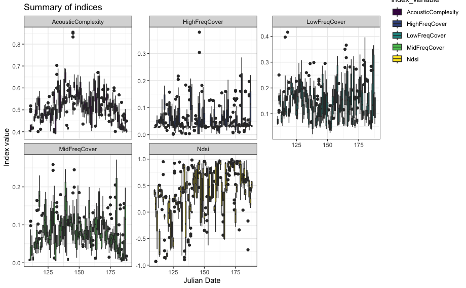
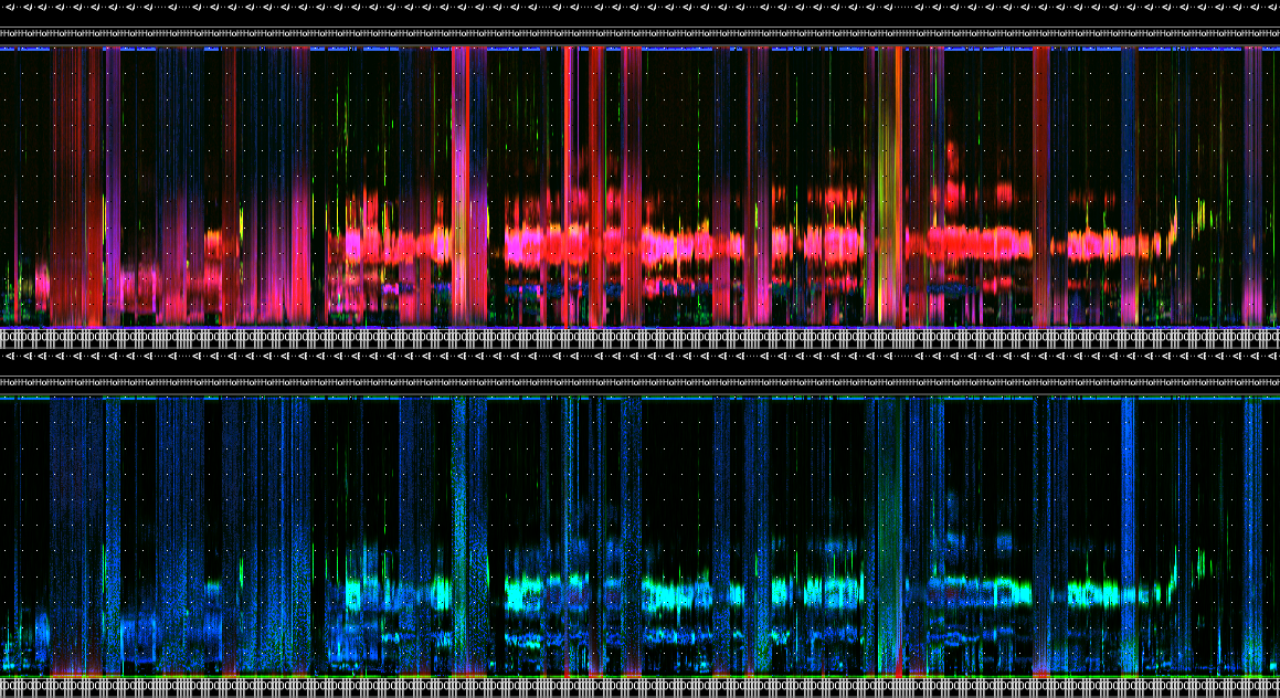
wt_run_ap(x = my_files, output_dir = paste0(root, 'ap_outputs'), path_to_ap = '/where/you/store/AP')

Then use wt_glean_ap() to plot the acoustic index and long-duration false-colour spectrogram (LDFC) results.

> # This example is from ABMI's Ecosystem Health Monitoring program
> 
> my_files <- wt_audio_scanner(".../ABMI-986-SE", file_type = "wav", extra_cols = )
> 
> wt_glean_ap(my_files %>% 
+                mutate(hour = lubridate::hour(recording_date_time)) %>%
+                filter(between(julian,110,220),
+                       hour %in% c(0:3,22:23)), input_dir = ".../ap_outputs", purpose = "biotic")
>

Applying a limited amplitude filter

We can use the wt_signal_level() function to search for sounds that exceed a certain amplitude threshold.

if (dir.exists(".")) {
  signal_file <- wt_audio_scanner(path = ".", file_type = "wav", extra_cols = T)
} else {
  'Can\'\t find this directory'
}

wt_signal_level(path = signal_file$file_path, 
                     fmin = 0, 
                     fmax = 10000, 
                     threshold = 5, 
                     channel = 'left')

# Run
s
# Return a list object, with parameters stored
str(s)

# We can view the output:
s['output']
# We have eleven detections that exceeded this threshold.

Linking data to WildTrax

Make tasks at any time using a wt_* standard data set with wt_make_aru_tasks().

wt_make_aru_tasks(input = files %>% select(-file_path), task_method = "1SPT", task_length = 180)

The function wt_songscope_tags() reformats the output obtained from a Wildlife Acoustics Songscope recognizer. This transformation involves converting the recognizer tags into tags that do not have a method type. This makes it possible to upload each hit as a tag in a task. Similarly, the function wt_kaleidoscope_tags() performs the same reformatting process, but with Kaleidoscope instead. It is worth noting that this function targeted for sonic and ultrasonic species upload.

# Convert Songscope output into WildTrax tags
wt_songscope_tags(
  input, 
  output = c("env", "csv"),
  my_output_file = NULL,
  species_code,
  vocalization_type,
  score_filter,
  method = c("USPM", "1SPT"),
  task_length
)

# Convert Kaleidoscope output into WildTrax tags
wt_kaleidoscope_tags(
  input, 
  output,
  tz, 
  freq_bump = T) # Add a frequency buffer to the tag, e.g. 20000 kHz

songscope_tags

If you’ve already uploaded recordings to WildTrax, scan your media using wt_audio_scanner() and a relative folder path.

my_files <- wt_audio_scanner(path = '/my/BigGrid/files', file_type = 'all', extra_cols = F)

And then download the project data you wish to compare it to:

my_projects <- wt_get_download_summary(sensor_id = 'ARU') %>%
  tibble::as_tibble() %>%
  filter(grepl('Big Grids',project)) %>% # Customized as needed
  mutate(data = purrr::map(.x = project_id, .f = ~wt_download_report(project_id = .x, sensor_id = 'ARU', weather_cols = F, reports = 'main')))

Alternatively, go to WildTrax to Organization > Recordings > Manage > Download Recordings to get a list of all recordings. Then either filter out or do an anti-join on location and recording_date_time. That should give you the remaining list of media that has not been processed or uploaded to WildTrax yet.