Acoustic pre-processing
acoustic-pre-processing.RmdThe following set of functions help to pre-process and organize audio and corresponding metadata. In conjunction, these tools allow you to select recordings parameterized to a specific study design.
Scanning audio files from a directory
The wt_audio_scanner() function reads in audio files
(either wac, wav or flac format) from a local directory and outputs
useful metadata.
wt_audio_scanner(path = ".", file_type = "wav", extra_cols = T)You might want to select recordings between certain times of day or year, or filter recordings based on some criteria.
files |>
dplyr::select(-file_path)Running the QUT Ecoacoustics AnalysisPrograms software on a wt_* standard data set
The wt_run_ap() function allows you to run the QUT
Analysis Programs (AP.exe) on your audio
data. AP generates acoustic index values and false-colour spectrograms
for each audio minute of data. Note that you must have the AP program
installed on your computer. See more with Towsey
et al. (2018).
# Use the wt_* tibble to execute the AP on the files
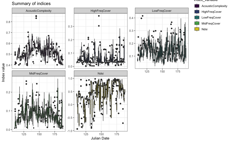
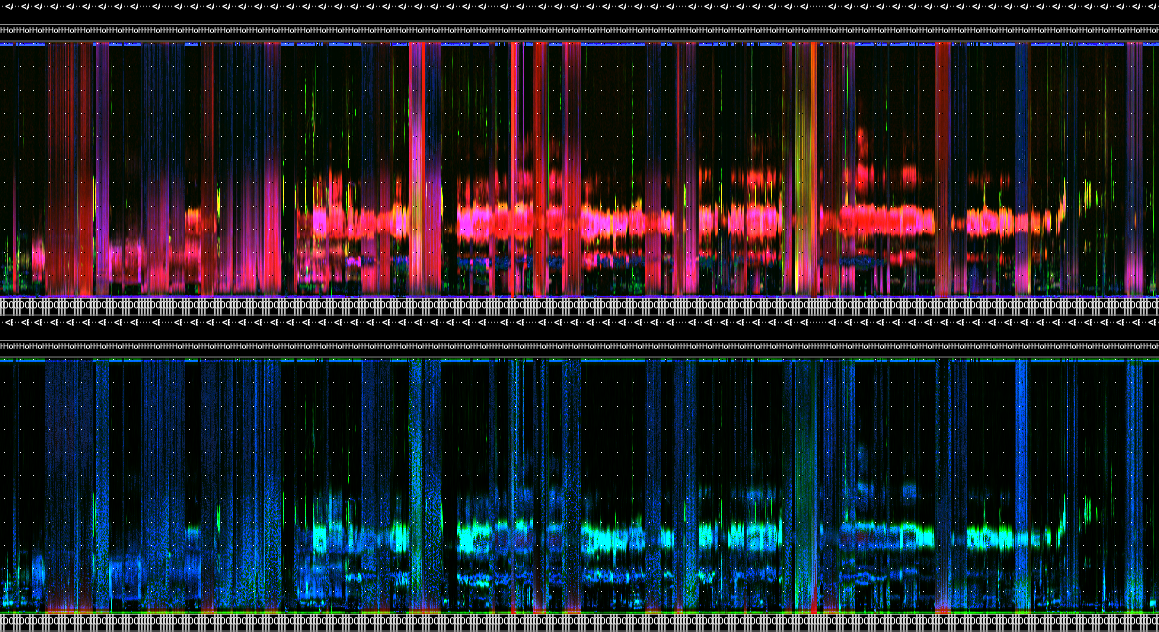
wt_run_ap(x = my_files, output_dir = paste0(root, 'ap_outputs'), path_to_ap = '/where/you/store/AP')Then use wt_glean_ap() to plot the acoustic index and
long-duration false-colour spectrogram (LDFC) results.
> # This example is from ABMI's Ecosystem Health Monitoring program
>
> my_files <- wt_audio_scanner(".../ABMI-986-SE", file_type = "wav", extra_cols = )
>
> wt_glean_ap(my_files |>
+                dplyr::mutate(hour = as.numeric(format(recording_date_time, "%H"))) |>
+                filter(between(julian,110,220),
+                       hour %in% c(0:3,22:23)), input_dir = ".../ap_outputs", purpose = "biotic")
> 
Applying a limited amplitude filter
We can use the wt_signal_level() function to search for
sounds that exceed a certain amplitude threshold.
if (dir.exists(".")) {
  signal_file <- wt_audio_scanner(path = ".", file_type = "wav", extra_cols = T)
} else {
  'Can\'\t find this directory'
}

wt_signal_level(path = signal_file$file_path,
                     fmin = 0,
                     fmax = 10000,
                     threshold = 5,
                     channel = 'left')
# Run
s
# Return a list object, with parameters stored
str(s)

# We can view the output:
s['output']
# We have eleven detections that exceeded this threshold.
Linking data to WildTrax
Make tasks at any time using a wt_* standard data set
with wt_make_aru_tasks().
wt_make_aru_tasks(input = files |>
                    select(-file_path), task_method = "1SPT", task_length = 180)
If you’ve already uploaded recordings to WildTrax, scan your media
using wt_audio_scanner() and a relative folder path.
my_files <- wt_audio_scanner(path = '/my/BigGrid/files', file_type = 'all', extra_cols = F)And then download the project data you wish to compare it to:
my_projects <- wt_get_projects("ARU") |>
  dplyr::filter(grepl("Cypress", project)) |>
  dplyr::pull(project_id) |>
  wt_download_report(sensor_id  = "ARU", reports = "main")
Alternatively use wt_get_sync("organization_recordings")
to get a list of all recordings. Then either filter out or do an
dplyr::anti_join() on location and recording_date_time.
That should give you the remaining list of media that has not been
processed or uploaded to WildTrax yet.
Integrating legacy data from classifiers
The wildrtrax package provides tools for integrating
classifier outputs from Wildlife Acoustics’ Kaleidoscope
and Songscope into
WildTrax-compatible data formats using the
wt_songscope_tags() and wt_kaleidoscope_tags()
functions. These functions convert classifier-generated detections into
WildTrax tags, allowing each detection to be uploaded as an individual
task-associated tag. This supports workflows where audio data have
already been processed by external classifiers, enabling existing
detections to be reformatted, aligned with media, and uploaded to
WildTrax for further review and analysis.
Here is some raw Songscope output:
# Convert Songscope output into WildTrax tags
readr::read_table("./CONI.txt")
#> # A tibble: 23 × 8
#> X:\\WLNP\\2018\\01\\WLNP-CONI\\…¹ `00:00:09.446` `0.192` `78` `20.7` `53.97`
#> <chr> <time> <dbl> <dbl> <dbl> <dbl>
#> 1 "X:\\WLNP\\2018\\01\\WLNP-CONI\\… 00'32" 0.192 75 23.3 56.0
#> 2 "X:\\WLNP\\2018\\01\\WLNP-CONI\\… 00'34" 0.205 77 27 53.2
#> 3 "X:\\WLNP\\2018\\01\\WLNP-CONI\\… 00'37" 0.218 69 23.1 54.2
#> 4 "X:\\WLNP\\2018\\01\\WLNP-CONI\\… 00'40" 0.269 67 36.1 50.1
#> 5 "X:\\WLNP\\2018\\01\\WLNP-CONI\\… 00'44" 0.269 69 26.4 60.7
#> 6 "X:\\WLNP\\2018\\01\\WLNP-CONI\\… 00'48" 0.218 73 25.8 50.8
#> 7 "X:\\WLNP\\2018\\01\\WLNP-CONI\\… 00'52" 0.371 71 63.8 50.4
#> 8 "X:\\WLNP\\2018\\01\\WLNP-CONI\\… 00'58" 0.256 63 33.1 54.2
#> 9 "X:\\WLNP\\2018\\01\\WLNP-CONI\\… 01'06" 0.422 73 64.9 52.2
#> 10 "X:\\WLNP\\2018\\01\\WLNP-CONI\\… 01'06" 0.333 68 36.2 55.1
#> # ℹ 13 more rows
#> # ℹ abbreviated name:
#> # ¹`X:\\WLNP\\2018\\01\\WLNP-CONI\\WLNP-CONI-001\\WLNP-CONI-001_20180720_203000.wav`
#> # ℹ 2 more variables: CONI_Boom2.0 <chr>, X8 <lgl>And here’s in the transformation with
wt_songscope_tags():
wt_songscope_tags(
  input = "./CONI.txt",
  output = "env",
  output_file = NULL,
  species = "CONI",
  vocalization = "SONG",
  score_filter = 10,
  method = "1SPT",
  duration = 180,
  sample_freq = 44100
)
Similarly, a Kaleidoscope output can be converted similarly:
wt_kaleidoscope_tags(
  input = "./id.csv",
  output = NULL,
  freq_bump = T) # Add a 20000 Hz frequency buffer to the tag