WildTrax APIs: Authentication, Endpoints, and Usage
apis.RmdOverview
The purpose of this vignette is to provide a clear introduction to accessing and interacting with WildTrax through our R package.
An API (Application Programming Interface) is a way for one program to communicate with another over the internet. In this case, the WildTrax APIs lets R talk to WildTrax servers to retrieve project data, recordings or tag information without using the website’s user interface manually.
wildrtrax wraps the WildTrax API in R
functions, so you can easily authenticate, request data, and work with
it in your analysis. You don’t have to write HTTP requests or handle
tokens directly as functions in the package handle these details and
provides user-friendly R functions to interact with WildTrax
programmatically.
Authenticating to WildTrax
Before accessing WildTrax data, you need to authenticate to obtain a token. This token lets the server recognize you and grant access to your data. Currently, authentication is done via Auth0 login (Google login is not supported). To simplify repeated use, store your WildTrax username and password as environment variables in R. This allows the package to securely use your credentials without requiring you to type them each time.
# Note that you need to use 'WT_USERNAME' and 'WT_PASSWORD'
Sys.setenv(WT_USERNAME = 'guest', WT_PASSWORD = 'Apple123')
Next, you use the wt_auth() function to
authenticate.
# Authenticate
wt_auth()
#> Authentication into WildTrax successful.
The Auth0 token you obtained will last for 12 hours. After that time, you will need to re-authenticate.
Making API calls
Once authenticated, you can now use various functions that call upon
the WildTrax APIs. For instance, you can use
wt_get_projects() to see basic metadata about projects that
you can download data for.
# Download the project summary you have access to
my_projects <- wt_get_projects('ARU')

head(my_projects)
#> # A tibble: 6 × 10
#>   organization_id organization_name project_sensor project_id project
#>             <int> <chr>             <chr>               <int> <chr>
#> 1            5351 CWS-ATL           ARU                   934 NF Breeding Bird …
#> 2            5350 CWS-PAC           ARU                  2187 Boreal Monitoring…
#> 3            5351 CWS-ATL           ARU                   935 Newfoundland Bree…
#> 4            5351 CWS-ATL           ARU                   924 Boreal Monitoring…
#> 5            5350 CWS-PAC           ARU                  2186 Boreal Monitoring…
#> 6            5396 Gov-QC            ARU                  1191 Suivi-BdQc 2021
#> # ℹ 5 more variables: project_status <chr>, project_creation_date <date>,
#> #   project_due_date <date>, task_count <int>, tasks_completed <int>
Using the project_id number in the download summary you can then use
wt_download_report() to access the species data. You can
also find the project_id number in the url of a WildTrax project,
e.g. https://portal.wildtrax.ca/home/aru-tasks.html?projectId=620&sensorId=ARU.
Corresponds to downloading the data from the Project dashboard like
illustrated below.
# Download the project report
my_report <- wt_download_report(project_id = 620, sensor_id = 'ARU', reports = "main")
head(my_report)
#> # A tibble: 6 × 31
#>   organization project_id location  location_id location_buffer_m longitude
#>   <chr>             <int> <chr>           <int>             <dbl>     <dbl>
#> 1 BU                  620 CHPP-WP-1       94515                NA     -110.
#> 2 BU                  620 CHPP-WP-1       94515                NA     -110.
#> 3 BU                  620 CHPP-WP-1       94515                NA     -110.
#> 4 BU                  620 CHPP-WP-1       94515                NA     -110.
#> 5 BU                  620 CHPP-WP-1       94515                NA     -110.
#> 6 BU                  620 CHPP-WP-1       94515                NA     -110.
#> # ℹ 25 more variables: latitude <dbl>, equipment_make <chr>,
#> #   equipment_model <chr>, recording_id <dbl>, recording_date_time <dttm>,
#> #   task_id <dbl>, task_is_complete <lgl>, task_duration <dbl>,
#> #   task_method <chr>, species_code <chr>, species_common_name <chr>,
#> #   species_scientific_name <chr>, individual_order <int>, tag_id <int>,
#> #   abundance <chr>, vocalization <chr>, detection_time <dbl>,
#> #   tag_duration <dbl>, rms_peak_dbfs <dbl>, tag_is_verified <lgl>, …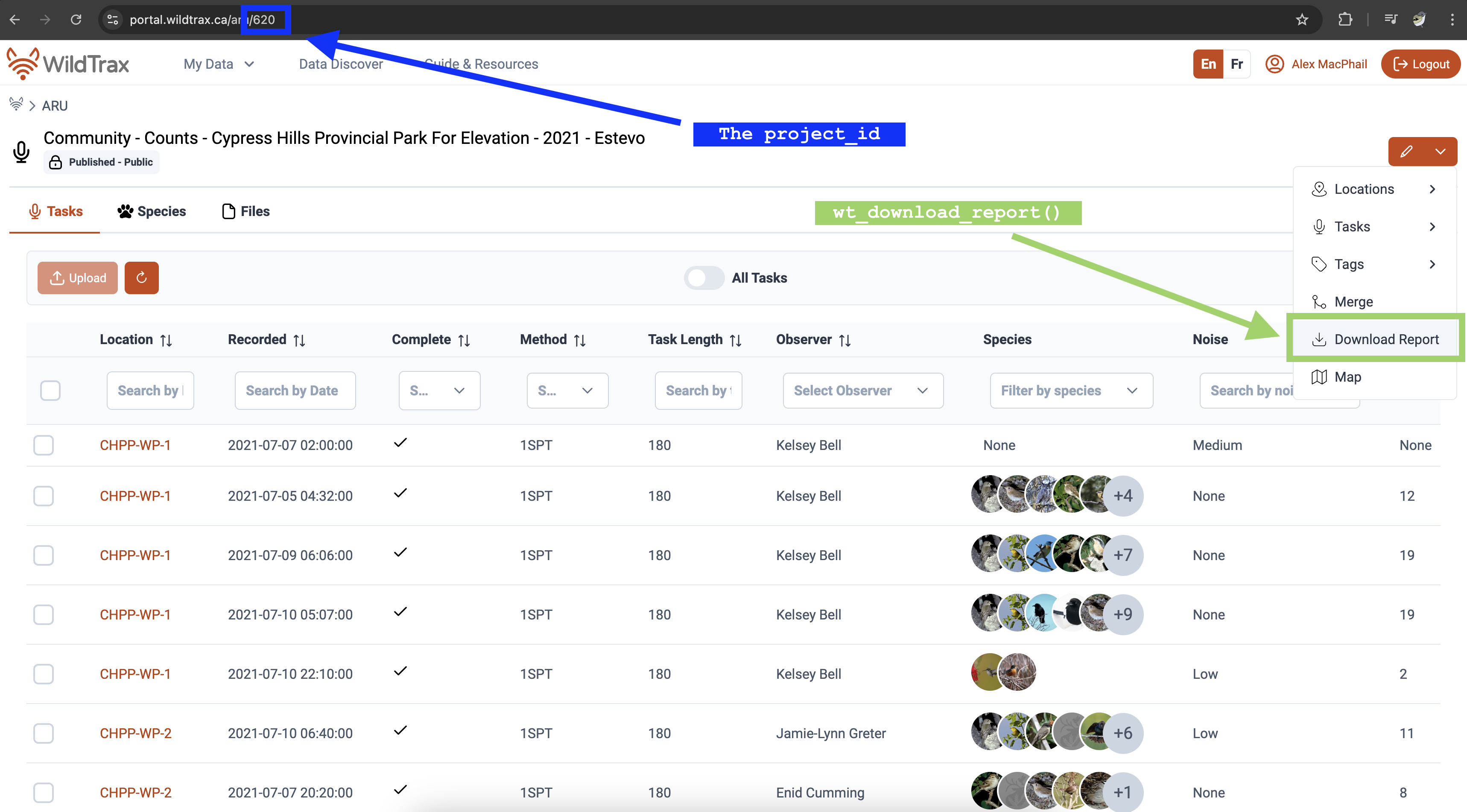
An easy way to download multiple projects at once is to use
wt_get_projects() and then filter by a substring in order
to get the project ids to download the data.
# Download all of the published Ecosystem Health ARU data to a single object
wt_get_projects("ARU") |>
  dplyr::filter(grepl("^Ecosystem Health",project)) %>%
  dplyr::mutate(data = purrr::map(.x = project_id, .f = ~wt_download_report(project_id = .x, sensor_id = "ARU", reports = "main")))
WildTrax also pre-formats ARU to point count (PC) data depending on the type of analysis you wish to perform. See the Boreal Avian Modelling project website and GitHub repositories to find out more on integration of avian point count and ARU data.
# As ARU format
my_report
#> # A tibble: 388 × 31
#>    organization project_id location  location_id location_buffer_m longitude
#>    <chr>             <int> <chr>           <int>             <dbl>     <dbl>
#>  1 BU                  620 CHPP-WP-1       94515                NA     -110.
#>  2 BU                  620 CHPP-WP-1       94515                NA     -110.
#>  3 BU                  620 CHPP-WP-1       94515                NA     -110.
#>  4 BU                  620 CHPP-WP-1       94515                NA     -110.
#>  5 BU                  620 CHPP-WP-1       94515                NA     -110.
#>  6 BU                  620 CHPP-WP-1       94515                NA     -110.
#>  7 BU                  620 CHPP-WP-1       94515                NA     -110.
#>  8 BU                  620 CHPP-WP-1       94515                NA     -110.
#>  9 BU                  620 CHPP-WP-1       94515                NA     -110.
#> 10 BU                  620 CHPP-WP-1       94515                NA     -110.
#> # ℹ 378 more rows
#> # ℹ 25 more variables: latitude <dbl>, equipment_make <chr>,
#> #   equipment_model <chr>, recording_id <dbl>, recording_date_time <dttm>,
#> #   task_id <dbl>, task_is_complete <lgl>, task_duration <dbl>,
#> #   task_method <chr>, species_code <chr>, species_common_name <chr>,
#> #   species_scientific_name <chr>, individual_order <int>, tag_id <int>,
#> #   abundance <chr>, vocalization <chr>, detection_time <dbl>, …
# As point count format
head(aru_as_pc)
#> # A tibble: 6 × 23
#>   organization project         project_id location location_id location_buffer_m
#>   <chr>        <chr>                <int> <chr>          <int>             <dbl>
#> 1 BU           Community - Co…        620 CHPP-WP…       94517                NA
#> 2 BU           Community - Co…        620 CHPP-WP…       94518                NA
#> 3 BU           Community - Co…        620 CHPP-WP…       89972                NA
#> 4 BU           Community - Co…        620 CHPP-WP…       89972                NA
#> 5 BU           Community - Co…        620 CHPP-WP…       89972                NA
#> 6 BU           Community - Co…        620 CHPP-WP…       89972                NA
#> # ℹ 17 more variables: latitude <dbl>, longitude <dbl>, survey_id <chr>,
#> #   survey_date <dttm>, survey_url <chr>, observer <chr>,
#> #   survey_distance_method <chr>, survey_duration_method <chr>,
#> #   detection_distance <chr>, detection_time <dbl>, species_code <chr>,
#> #   species_common_name <chr>, species_scientific_name <chr>,
#> #   individual_count <chr>, detection_heard <lgl>, detection_seen <lgl>,
#> #   detection_comments <chr>
Species
Downloading the WildTrax species table with
wt_get_species() also grants you access to other valuable
columns or provides a complete list of the species currently supported
by WildTrax.
# Download the WildTrax species table
wt_get_species() |> arrange(species_code)
You can also determine which species are allowed in and out of
projects via the wt_get_project_species() function. The
included column will expose which species have been
currently tagged in the Project.
my_project_species <- wt_get_project_species(620)

my_project_species |>
  filter(included == TRUE)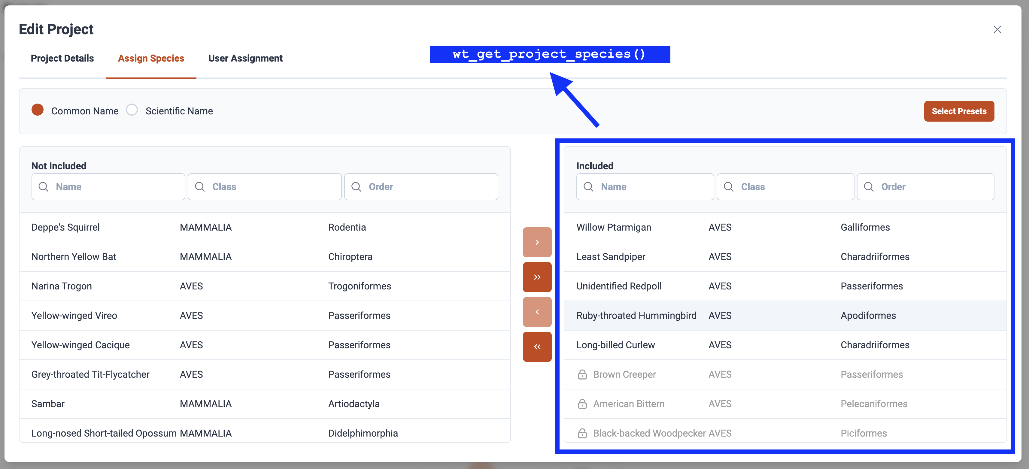
Data Discover
Explore species and data within WildTrax’s Data Discover by employing the
wt_dd_summary() function. Access a portion of data, even
without user privileges. Utilize wt_auth() to uncover data
pertinent to your account or those publicly available on WildTrax.
discover <- wt_dd_summary(sensor = "ARU", species = "White-throated Sparrow", boundary = NULL)
head(discover)
#> $`lat-long-summary`
#> # A tibble: 11 × 5
#> projectId project_name count species_common_name species_scientific_n…¹
#> <int> <chr> <dbl> <chr> <chr>
#> 1 31 "BU-Community - C… 1232 White-throated Spa… Zonotrichia albicollis
#> 2 1855 "CWS-ONT-Ontario … 1126 White-throated Spa… Zonotrichia albicollis
#> 3 41 "BU-Community - C… 829 White-throated Spa… Zonotrichia albicollis
#> 4 1070 "CWS-ONT-Ontario … 805 White-throated Spa… Zonotrichia albicollis
#> 5 3139 "CWS-ONT-Ontario … 601 White-throated Spa… Zonotrichia albicollis
#> 6 659 "CWS-ONT-Ontario … 528 White-throated Spa… Zonotrichia albicollis
#> 7 2821 "CWS-ONT-Ontario … 469 White-throated Spa… Zonotrichia albicollis
#> 8 1 "ABMI-Ecosystem H… 343 White-throated Spa… Zonotrichia albicollis
#> 9 19 "ABMI-Ecosystem H… 291 White-throated Spa… Zonotrichia albicollis
#> 10 142 "ABMI-Ecosystem H… 280 White-throated Spa… Zonotrichia albicollis
#> 11 NA "" 8096 White-throated Spa… Zonotrichia albicollis
#> # ℹ abbreviated name: ¹species_scientific_name
#>
#> $`map-projects`
#> # A tibble: 11,654 × 4
#> species_common_name count longitude latitude
#> <chr> <int> <dbl> <dbl>
#> 1 White-throated Sparrow 1 -125. 56.1
#> 2 White-throated Sparrow 1 -125. 56.1
#> 3 White-throated Sparrow 1 -125. 56.1
#> 4 White-throated Sparrow 1 -125. 56.1
#> 5 White-throated Sparrow 1 -125. 56.2
#> 6 White-throated Sparrow 1 -124. 55.6
#> 7 White-throated Sparrow 1 -124. 56.1
#> 8 White-throated Sparrow 1 -124. 56.1
#> 9 White-throated Sparrow 1 -124. 56.1
#> 10 White-throated Sparrow 1 -124. 56.1
#> # ℹ 11,644 more rowsUse custom bounding areas:
# Define a polygon
my_aoi <- list(
  c(-113.96068, 56.23817),
  c(-117.06285, 54.87577),
  c(-112.88035, 54.90431),
  c(-113.96068, 56.23817)
)

discover_with_aoi <- wt_dd_summary(sensor = "ARU", species = "White-throated Sparrow", boundary = my_aoi)

head(discover_with_aoi)
library(sf)
# Alberta bounding box
abbox <- read_sf("...shp") |> # Shapefile of Alberta
  filter(Province == "Alberta") |>
  st_transform(crs = 4326) |>
  st_bbox()

discover <- wt_dd_summary(sensor = "ARU", species = "White-throated Sparrow", boundary = abbox)

head(discover)
Accessing WildTrax data with wt_get_sync() and
wt_get_view()
wt_get_sync() and wt_get_view() provide
programmatic access to WildTrax data through various APIs.
wt_get_sync() interfaces with the synchronization (sync)
endpoints, which expose data associated with Organizations and Projects.
These endpoints return data objects related to locations, visits,
deployments, equipment, project tasks, and tags. The sync APIs are
primarily intended for workflows that require advanced or batch
manipulation. wt_get_view() provides access to the user
interface views and tables that present structured representations of
WildTrax data. These views are optimized for reporting and analysis and
may aggregate or normalize information. Used together,
wt_get_sync() and wt_get_view() allow users to
retrieve operational data from the WildTrax system and work with
analysis-ready representations of those data within R.
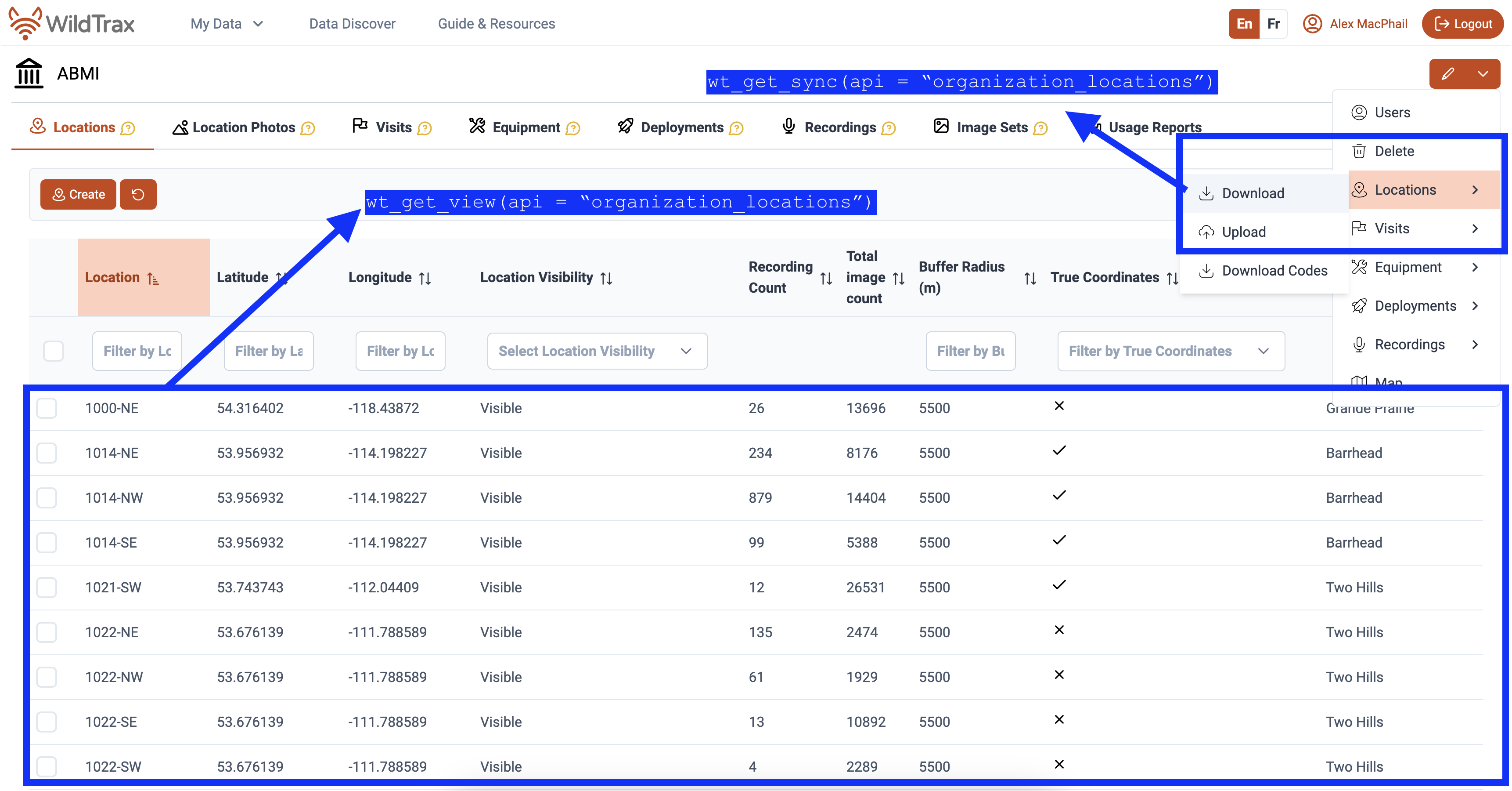
# Extracting location information from all API functions

# All location information from Organization location sync
wt_get_sync(api = "organization_locations", organization = 5205)

# All location information from Locations tab
wt_get_view(api = "organization_locations", organization = 5205)

# All location information from Project location sync
wt_get_sync(api = "project_locations", project = 326)

wt_download_report(project_id = 326, sensor_id = 'ARU', reports = 'location')