library(sciSpatialR)
library(terra)
#> terra 1.9.50
library(sf)
#> Linking to GEOS 3.12.1, GDAL 3.8.4, PROJ 9.4.0; sf_use_s2() is TRUE
Four ways to give a point a value
| Question | Call | Returns |
|---|---|---|
| What is the value at this location? | extract_points() |
one column per raster layer |
| What is the average (or sum, or spread) around it? | extract_buffer() |
one column per layer × radius |
| What is the composition around it? | extract_proportion() |
one column per class |
| Which polygon is it in? | extract_vector() |
the polygon’s attributes |
The first three read rasters and return a plain
data.frame; the last reads a polygon layer and returns an
sf
Layers and points to extract from
Everything below runs on synthetic layers built on the reference grid, so this vignette needs no external data.
Working from the share instead, list_variables() is a
way to decide what to extract before extracting it. A catalogued product
is often a stack of dozens of bands — SoilGrids alone publishes 61 — and
the function reports what each one measures, its units, and its valid
range, so the columns can be chosen by name rather than by opening the
raster and counting layers:
list_variables(product = "soilgrids_250_v2_ab")

# Or across the whole catalogue, searched by what a band measures.
v <- list_variables(verbose = FALSE)
v[grepl("pH", v$measure, fixed = TRUE), c("name", "band", "units")]
Band names line up with the layer names extract_points()
returns, so the two read together. The catalogue vignette covers the rest of those
functions.
Back to the synthetic layers: a continuous surface standing in for a canopy height model, and a four-class categorical layer derived from it:
set.seed(42)

ref   <- ab_grid()
east  <- init(ref, "x")
north <- init(ref, "y")

chm <- 14 +
  6 * sin(east / 70000) * cos(north / 110000) -
  4 * (north - 5.4e6) / 1.2e6
chm <- chm + init(ref, function(n) rnorm(n, 0, 1.5))
chm <- mask(chm, ref)
names(chm) <- "canopy_height"

cover <- classify(
  chm,
  matrix(
    c(-Inf,  8, 1,
         8, 14, 2,
        14, 18, 3,
        18, Inf, 4),
    ncol = 3, byrow = TRUE
  )
)
names(cover) <- "cover"
cover
#> class       : SpatRaster
#> size        : 1234, 695, 1  (nrow, ncol, nlyr)
#> resolution  : 1000, 1000  (x, y)
#> extent      : 170616.2, 865616.2, 5425532, 6659532  (xmin, xmax, ymin, ymax)
#> coord. ref. : NAD83 / Alberta 10-TM (Forest) (EPSG:3400)
#> source(s)   : memory
#> varname     : grid_1km
#> name        : cover
#> min value   :     1
#> max value   :     4
plot(chm)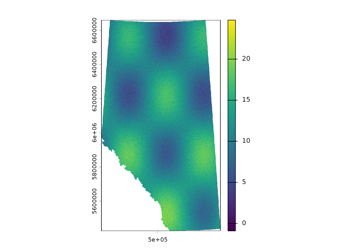
plot(cover)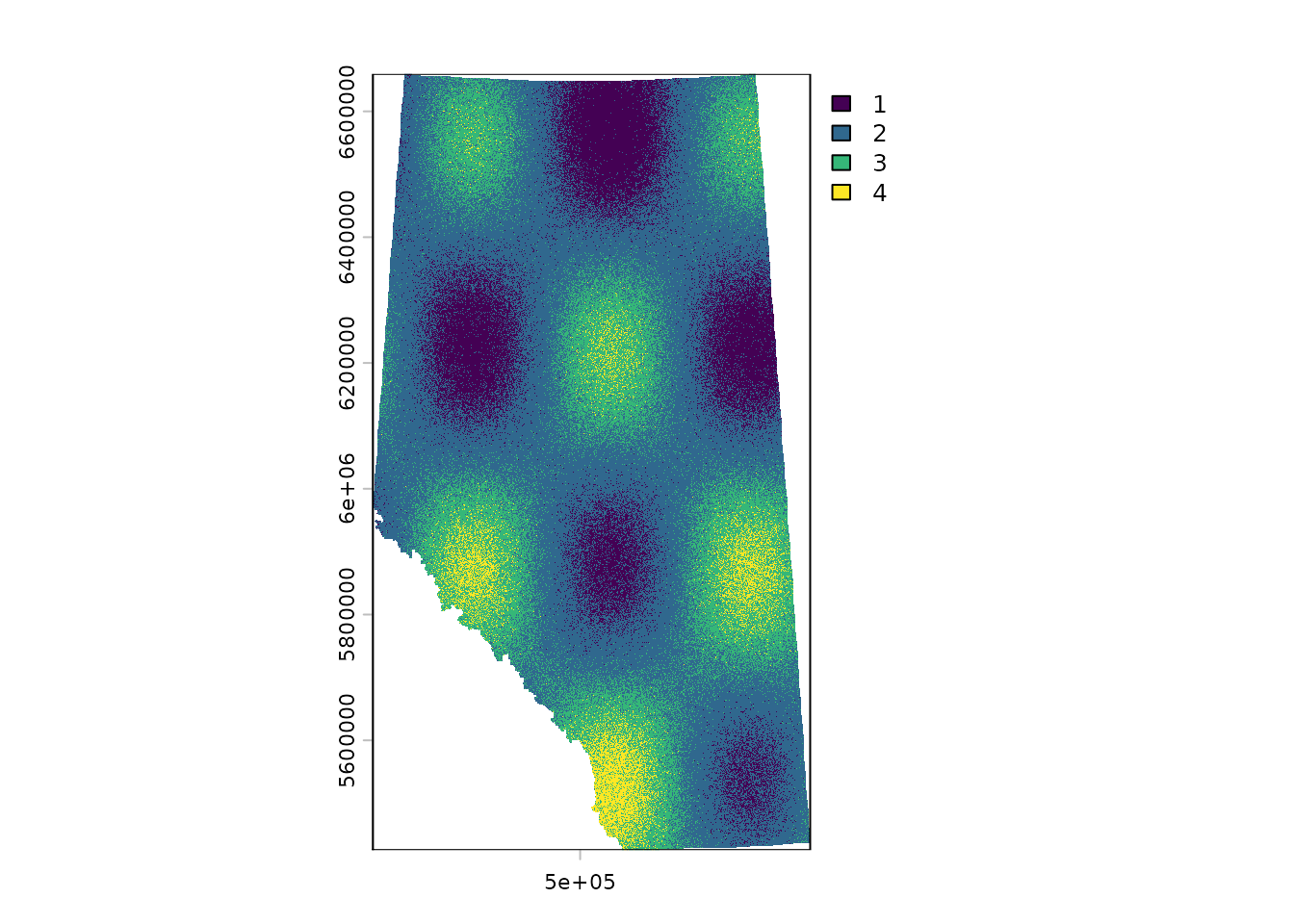
Both are masked to Alberta, which matters later: cells outside the
province are NA, and a buffer near the border will contain
some of them.
The survey locations are five sites in geographic coordinates — the state point data usually arrives in, straight off a GPS or out of a database:
sites <- st_as_sf(
  data.frame(
    site = c("calgary", "edmonton", "fort_mcmurray",
             "grande_prairie", "border"),
    x = c(-114.07, -113.49, -111.38, -118.80, -119.90),
    y = c(  51.05,   53.55,   56.73,    55.17,    54.00)
  ),
  coords = c("x", "y"),
  crs    = 4326
)
sites
#> Simple feature collection with 5 features and 1 field
#> Geometry type: POINT
#> Dimension:     XY
#> Bounding box:  xmin: -119.9 ymin: 51.05 xmax: -111.38 ymax: 56.73
#> Geodetic CRS:  WGS 84
#>             site              geometry
#> 1        calgary POINT (-114.07 51.05)
#> 2       edmonton POINT (-113.49 53.55)
#> 3  fort_mcmurray POINT (-111.38 56.73)
#> 4 grande_prairie  POINT (-118.8 55.17)
#> 5         border     POINT (-119.9 54)
border sits close to the British Columbia line and is
there to show what happens at the edge of a masked layer:
# Reprojected inline for the plot only; the extraction sections
# below do it properly with `harmonize_crs()`.
sites_xy <- st_coordinates(harmonize_crs(sites, warn = FALSE))

plot(chm)
points(sites_xy, pch = 21, bg = "white", cex = 1.2)

# Label eastern sites on their left so nothing runs off the panel.
label_side <- ifelse(
  sites_xy[, "X"] > mean(range(sites_xy[, "X"])), 2, 4
)
text(sites_xy, labels = sites$site, pos = label_side, cex = 0.7)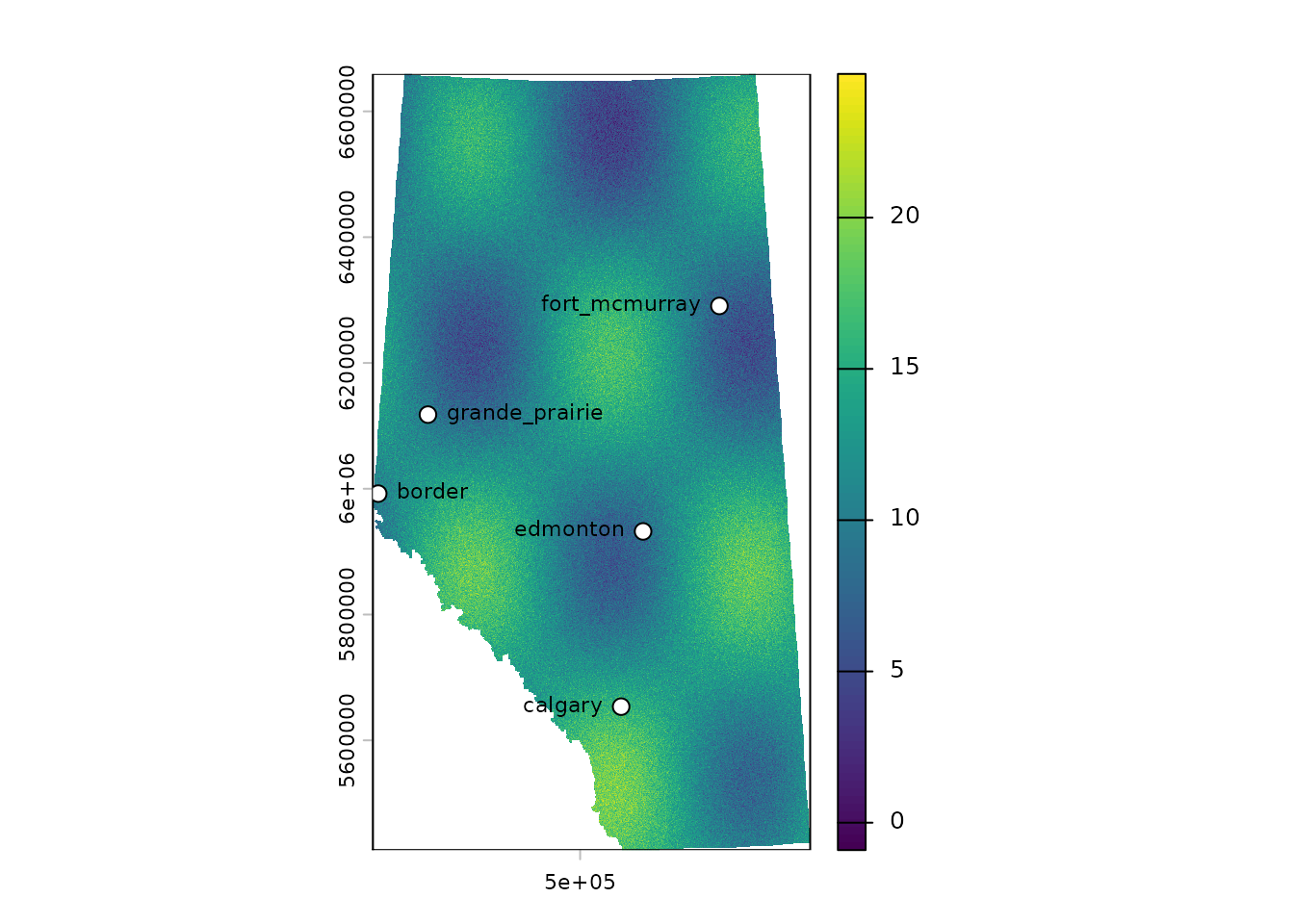
extract_points()
The value of the cell each point falls in:
extract_points(chm, sites)
#> Warning in extract_points(chm, sites): CRS mismatch: reprojecting `points` to
#> raster CRS.
#>             site canopy_height
#> 1        calgary     17.349996
#> 2       edmonton      5.261704
#> 3  fort_mcmurray      6.798836
#> 4 grande_prairie      6.822229
#> 5         border     11.324230
Note what did not have to happen first. The points are in EPSG:4326 and the raster is in Alberta 10-TM, so the function reprojected the points and warned about it. The warning is deliberate — reprojecting silently is how a point set ends up somewhere unintended — but it is noise once the reprojection is known to be right. Harmonize first and the call is quiet:
sites_ab <- harmonize_crs(sites)
#> Reprojecting `points` to the reference grid CRS (NAD83 / Alberta 10-TM (Forest)).
extract_points(chm, sites_ab)
#>             site canopy_height
#> 1        calgary     17.349996
#> 2       edmonton      5.261704
#> 3  fort_mcmurray      6.798836
#> 4 grande_prairie      6.822229
#> 5         border     11.324230
The result is a data.frame, not an
sf. bind = TRUE column-binds the
extracted values to the attributes of points, and
the geometry is dropped along the way. That is usually what a modelling
table wants; when the geometry is needed too, bind the values back onto
the sf object yourself:
vals      <- extract_points(chm, sites_ab, bind = FALSE)
sites_val <- cbind(sites_ab, vals)
class(sites_val)
#> [1] "sf"         "data.frame"
bind = FALSE returns just the extracted columns, in the
same row order as points, which is what makes that
cbind safe.
Multi-layer rasters give one column per layer, so a stack of prepared covariates is one call:
covariates <- c(chm, cover)
extract_points(covariates, sites_ab)
#>             site canopy_height cover
#> 1        calgary     17.349996     3
#> 2       edmonton      5.261704     1
#> 3  fort_mcmurray      6.798836     1
#> 4 grande_prairie      6.822229     1
#> 5         border     11.324230     2
Arguments in ... reach terra::extract().
The useful one is method: the default "simple"
takes the value of the containing cell, while "bilinear"
interpolates from the four nearest cell centres, which is smoother for a
continuous surface and meaningless for class codes.
extract_points(chm, sites_ab, method = "bilinear")
#>             site canopy_height
#> 1        calgary     17.237045
#> 2       edmonton      5.559297
#> 3  fort_mcmurray      6.460034
#> 4 grande_prairie      7.773671
#> 5         border     11.064706
A point outside the layer’s data — off the extent, or on a masked
cell — returns NA rather than an error:
off <- st_as_sf(
  data.frame(site = "saskatoon", x = -106.67, y = 52.13),
  coords = c("x", "y"), crs = 4326
)
extract_points(chm, harmonize_crs(off, warn = FALSE))
#>        site canopy_height
#> 1 saskatoon            NA
That NA is worth checking for after every extraction. It
means one of two very different things — the point is outside the study
area, or the layer has a hole in it.
extract_buffer()
A point value describes one 1 km cell. Most covariates in a species
model are not that: bird detections respond to the forest
around the station, not the pixel under it.
extract_buffer() summarises the cells whose centres fall
within a circular buffer, and is vectorised over radii so a whole
multi-scale set comes back in one table:
extract_buffer(chm, sites_ab, radii = c(1000, 5000, 20000))
#>             site canopy_height_r1000_mean canopy_height_r5000_mean
#> 1        calgary                17.323679                15.751265
#> 2       edmonton                 6.118019                 8.365948
#> 3  fort_mcmurray                 6.147757                 7.168125
#> 4 grande_prairie                 9.365725                 9.766332
#> 5         border                10.851850                10.223140
#>   canopy_height_r20000_mean
#> 1                 15.607988
#> 2                  8.325852
#> 3                  7.322629
#> 4                  9.788987
#> 5                       NaN
Radii are in the CRS units — metres here, because
ab_crs() is projected. The columns are named
<layer>_r<radius>_<fun>, so several
radii, several layers, and several summary functions can coexist in one
table without collision.
Look at the border row: the two smaller radii came back
fine and the 20 km one did not. That buffer reaches across the
provincial line into cells that are NA in a masked layer,
and a mean over anything containing an NA is not a number.
Arguments in ... are forwarded to the summary function, so
na.rm = TRUE fixes it:
extract_buffer(chm, sites_ab, radii = c(1000, 5000, 20000),
               na.rm = TRUE)
#>             site canopy_height_r1000_mean canopy_height_r5000_mean
#> 1        calgary                17.323679                15.751265
#> 2       edmonton                 6.118019                 8.365948
#> 3  fort_mcmurray                 6.147757                 7.168125
#> 4 grande_prairie                 9.365725                 9.766332
#> 5         border                10.851850                10.223140
#>   canopy_height_r20000_mean
#> 1                 15.607988
#> 2                  8.325852
#> 3                  7.322629
#> 4                  9.788987
#> 5                 10.543791
This is the argument to think about rather than to always
pass. na.rm = TRUE means “summarise the part of
the buffer I have data for”. To see how much of the buffer you have,
extract a count of valid pixels within each buffer:
extract_buffer(chm, sites_ab, radii = 20000,
               fun = function(v, ...) sum(!is.na(v)),
               fun_name = "n_valid")
#>             site canopy_height_r20000_n_valid
#> 1        calgary                         1250
#> 2       edmonton                         1249
#> 3  fort_mcmurray                         1253
#> 4 grande_prairie                         1250
#> 5         border                          907
A 20 km buffer on a 1 km grid covers roughly 1,250 cells; anything much below that is a buffer that has left the layer.
Two things about that call. fun is any function that
reduces a vector to one number, so sd, max,
median, or a custom one all work. And fun_name
supplies the column suffix: a named function is labelled from its own
name, but an inline function has no name to take, so pass one rather
than letting it fall back to stat.
extract_buffer(chm, sites_ab, radii = 5000, fun = sd, na.rm = TRUE)
#>             site canopy_height_r5000_sd
#> 1        calgary               1.519455
#> 2       edmonton               1.612942
#> 3  fort_mcmurray               1.679334
#> 4 grande_prairie               1.357974
#> 5         border               1.408534
Radius is a modelling choice, not a technical one, and
extract_buffer allows for multiple radii.
multi <- extract_buffer(covariates, sites_ab,
                        radii = c(5000, 20000), na.rm = TRUE)
names(multi)
#> [1] "site"                      "canopy_height_r5000_mean"
#> [3] "cover_r5000_mean"          "canopy_height_r20000_mean"
#> [5] "cover_r20000_mean"
Note cover_r5000_mean in there. It is the mean of the
class codes 1–4, which is not a quantity — the mean of “wetland” and
“upland” does not exist. Categorical layers need the next function.
extract_proportion()
For a categorical layer, the meaningful summary within a buffer is
composition: how much of each class. extract_proportion()
returns one column per class, and one row per point:
extract_proportion(cover, sites_ab, radius = 10000)
#>             site    cover_1   cover_2     cover_3    cover_4
#> 1        calgary 0.00000000 0.1401274 0.808917197 0.05095541
#> 2       edmonton 0.40514469 0.5948553 0.000000000 0.00000000
#> 3  fort_mcmurray 0.68888889 0.3111111 0.000000000 0.00000000
#> 4 grande_prairie 0.14935065 0.8441558 0.006493506 0.00000000
#> 5         border 0.06737589 0.9255319 0.007092199 0.00000000
Each row sums to one:
props <- extract_proportion(cover, sites_ab, radius = 10000,
                            bind = FALSE)
rowSums(props)
#> [1] 1 1 1 1 1
It sums to one for border as well, even though 16 of the
298 cells in that buffer are outside the province. Proportions are of
the valid cells in the buffer — NA cells are
dropped before the tabulation rather than counted as a class — which is
the same decision na.rm = TRUE makes in
extract_buffer(), taken for you because there is no
sensible alternative. The consequence is the same caveat: a proportion
says nothing about how much data it was computed from. Pair it with a
count of valid pixels when a buffer might be mostly missing.
Radius changes the answer, and a small one concentrates it on the class under the point — a 2 km buffer on a 1 km grid is about a dozen cells, so the proportions are coarse fractions of a small denominator:
extract_proportion(cover, sites_ab, radius = 2000)
#>             site    cover_1   cover_2   cover_3
#> 1        calgary 0.00000000 0.1666667 0.8333333
#> 2       edmonton 0.54545455 0.4545455 0.0000000
#> 3  fort_mcmurray 0.69230769 0.3076923 0.0000000
#> 4 grande_prairie 0.20000000 0.8000000 0.0000000
#> 5         border 0.09090909 0.9090909 0.0000000
extract_proportion(cover, sites_ab, radius = 10000)
#>             site    cover_1   cover_2     cover_3    cover_4
#> 1        calgary 0.00000000 0.1401274 0.808917197 0.05095541
#> 2       edmonton 0.40514469 0.5948553 0.000000000 0.00000000
#> 3  fort_mcmurray 0.68888889 0.3111111 0.000000000 0.00000000
#> 4 grande_prairie 0.14935065 0.8441558 0.006493506 0.00000000
#> 5         border 0.06737589 0.9255319 0.007092199 0.00000000
Two constraints follow from how the columns are built, and the table above has already shown one of them.
The columns are the classes observed across the buffers, not
the classes in the layer. cover_4 is in the 10 km
table and gone from the 2 km one: no 2 km buffer happened to contain
that class. Two runs on different point sets can therefore come back
with different columns, which will misalign silently if you
rbind them or feed them to a model fitted on the other set.
A single site is the extreme case:
one <- extract_proportion(cover, sites_ab[1, ], radius = 2000,
                          bind = FALSE)
names(one)
#> [1] "cover_2" "cover_3"
names(props)
#> [1] "cover_1" "cover_2" "cover_3" "cover_4"
When that matters, reconcile the columns yourself against the full class set of the layer:
classes  <- sort(unique(values(cover, na.rm = TRUE)))
expected <- paste0("cover_", classes)
missing  <- setdiff(expected, names(one))
one[missing] <- 0
one[expected]
#>   cover_1   cover_2   cover_3 cover_4
#> 1       0 0.1666667 0.8333333       0
The layer must be a single band. Class proportions for a stack would need one column set per layer, which the return shape has no room for, so it errors rather than guessing:
extract_proportion(covariates, sites_ab, radius = 5000)
#> Error in `extract_proportion()`:
#> ! `x` must be a single-layer SpatRaster.
Call it once per categorical layer and cbind the results
— and note that radius is a single number too, so multiple
scales are multiple calls, unlike extract_buffer().
extract_vector()
The last question is a join rather than a summary: which polygon does this point fall in? Natural subregion, LUF zone, land ownership, watershed — anything that arrives as a polygon layer with attributes.
The demonstration layer is a synthetic set of management zones covering the province:
zones <- st_sf(
  zone_id   = 1:6,
  zone_name = c("southwest", "southeast", "central_west",
                "central_east", "northwest", "northeast"),
  crew      = c("A", "A", "B", "B", "C", "C"),
  geometry  = st_make_grid(st_as_sf(ab_boundary()), n = c(2, 3))
)
zones
#> Simple feature collection with 6 features and 3 fields
#> Geometry type: POLYGON
#> Dimension:     XY
#> Bounding box:  xmin: 170844.3 ymin: 5425575 xmax: 865133.5 ymax: 6659344
#> Projected CRS: NAD83 / Alberta 10-TM (Forest)
#>   zone_id    zone_name crew                       geometry
#> 1       1    southwest    A POLYGON ((170844.3 5425575,...
#> 2       2    southeast    A POLYGON ((517988.9 5425575,...
#> 3       3 central_west    B POLYGON ((170844.3 5836832,...
#> 4       4 central_east    B POLYGON ((517988.9 5836832,...
#> 5       5    northwest    C POLYGON ((170844.3 6248088,...
#> 6       6    northeast    C POLYGON ((517988.9 6248088,...
extract_vector(sites_ab, zones)
#> Simple feature collection with 5 features and 4 fields
#> Geometry type: POINT
#> Dimension:     XY
#> Bounding box:  xmin: 179056.2 ymin: 5653533 xmax: 721350 ymax: 6290665
#> Projected CRS: NAD83 / Alberta 10-TM (Forest)
#>             site zone_id    zone_name crew                 geometry
#> 1        calgary       2    southeast    A   POINT (565161 5653533)
#> 2       edmonton       4 central_east    B POINT (600000.9 5932142)
#> 3  fort_mcmurray       6    northeast    C   POINT (721350 6290665)
#> 4 grande_prairie       3 central_west    B POINT (258107.1 6117851)
#> 5         border       3 central_west    B POINT (179056.2 5992241)
Three differences from the raster extractors:
It is sf in, sf out. Both
arguments must be sf objects and the geometry survives,
because a spatial join is sf::st_join() underneath and the
points keep their own geometry column. That also means the result can be
passed straight into another extract_vector() call, or
written to a GeoPackage.
It handles the CRS the other way round. The raster functions reproject the points to the raster; this one reprojects the polygons to the points, so the output geometry is always in the CRS the points arrived in. Passing the unprojected points gives the same join, in EPSG:4326:
st_crs(extract_vector(sites, zones))$input
#> [1] "EPSG:4326"
cols trims the join. A subregion layer
with forty attribute columns will otherwise drag all forty into the
modelling table:
extract_vector(sites_ab, zones, cols = "zone_name")
#> Simple feature collection with 5 features and 2 fields
#> Geometry type: POINT
#> Dimension:     XY
#> Bounding box:  xmin: 179056.2 ymin: 5653533 xmax: 721350 ymax: 6290665
#> Projected CRS: NAD83 / Alberta 10-TM (Forest)
#>             site    zone_name                 geometry
#> 1        calgary    southeast   POINT (565161 5653533)
#> 2       edmonton central_east POINT (600000.9 5932142)
#> 3  fort_mcmurray    northeast   POINT (721350 6290665)
#> 4 grande_prairie central_west POINT (258107.1 6117851)
#> 5         border central_west POINT (179056.2 5992241)
A name that is not in polygons is dropped rather than
flagged, so a typo costs you a column silently — check the result’s
names, or cols against names(polygons), rather
than trusting the call:
names(extract_vector(sites_ab, zones, cols = c("zone_name", "zoen")))
#> [1] "site"      "zone_name" "geometry"
Two failure modes
First, a point outside every polygon joins to NA,
because the underlying join is a left join — the row survives, the
attributes do not:
extract_vector(harmonize_crs(off, warn = FALSE), zones)
#> Simple feature collection with 1 feature and 4 fields
#> Geometry type: POINT
#> Dimension:     XY
#> Bounding box:  xmin: 1069474 ymin: 5805966 xmax: 1069474 ymax: 5805966
#> Projected CRS: NAD83 / Alberta 10-TM (Forest)
#>        site zone_id zone_name crew                geometry
#> 1 saskatoon      NA      <NA> <NA> POINT (1069474 5805966)
That is the right default for a modelling table, where a dropped row
is worse than a visible NA. sf::st_join()
arguments reach through ..., so left = FALSE
turns it into an inner join when you would rather lose the row:
nrow(extract_vector(harmonize_crs(off, warn = FALSE), zones,
                    left = FALSE))
#> [1] 0
Second, a point inside overlapping polygons is returned once per match, so the result can be longer than the input:
overlapping <- st_sf(
  layer    = c("survey_2019", "survey_2024"),
  geometry = c(
    st_as_sfc(st_bbox(zones)),
    st_as_sfc(st_bbox(zones))
  ),
  crs = st_crs(zones)
)
nrow(sites_ab)
#> [1] 5
nrow(extract_vector(sites_ab, overlapping))
#> [1] 10
Nested or overlapping polygon layers are common — protected areas
inside land-use zones, historical survey footprints — so check
nrow() against the input rather than assuming a one-to-one
join.
st_join()’s largest = TRUE collapses the
duplicates back to one row per point, but read what it does before
reaching for it: it keeps the match with the largest area of overlap,
and a point has no area, so every candidate ties and the winner
is whichever polygon comes first in the layer. Here that is the outer
zone in one ordering and the inner zone in the other:
nested <- st_sf(
  zone     = c("outer", "inner"),
  geometry = st_sfc(
    st_as_sfc(st_bbox(zones))[[1]],
    st_buffer(st_geometry(sites_ab)[1], 50000)[[1]],
    crs = st_crs(zones)
  )
)

extract_vector(sites_ab[1, ], nested, largest = TRUE)$zone
#> Warning: attribute variables are assumed to be spatially constant throughout
#> all geometries
#> [1] "outer"
extract_vector(sites_ab[1, ], nested[2:1, ], largest = TRUE)$zone
#> Warning: attribute variables are assumed to be spatially constant throughout
#> all geometries
#> [1] "inner"
It is a deduplication, not a resolution. When one of the polygons is the right answer — the subregion rather than the survey footprint — subset the polygon layer before the join instead.
A worked pipeline
The four together, as they would appear in a modelling pipeline — a point set and a stack of prepared layers going in, one modelling table coming out:
# 1. Points into the reference CRS, once, up front
survey <- harmonize_crs(sites)
#> Reprojecting `points` to the reference grid CRS (NAD83 / Alberta 10-TM (Forest)).

# 2. Point-in-cell values for the continuous layers
at_point <- extract_points(chm, survey, bind = FALSE)

# 3. Multi-scale neighbourhood summaries
around <- extract_buffer(chm, survey, radii = c(1000, 5000),
                         na.rm = TRUE, bind = FALSE)

# 4. Composition of the categorical layer at the larger scale
comp <- extract_proportion(cover, survey, radius = 5000,
                           bind = FALSE)

# 5. Which management zone each site is in
in_zone <- extract_vector(survey, zones, cols = "zone_name")

# 6. One table
model_data <- cbind(
  st_drop_geometry(in_zone),
  at_point, around, comp
)
model_data
#>             site    zone_name canopy_height canopy_height_r1000_mean
#> 1        calgary    southeast     17.349996                17.323679
#> 2       edmonton central_east      5.261704                 6.118019
#> 3  fort_mcmurray    northeast      6.798836                 6.147757
#> 4 grande_prairie central_west      6.822229                 9.365725
#> 5         border central_west     11.324230                10.851850
#>   canopy_height_r5000_mean    cover_1   cover_2 cover_3 cover_4
#> 1                15.751265 0.00000000 0.1250000     0.8   0.075
#> 2                 8.365948 0.35064935 0.6493506     0.0   0.000
#> 3                 7.168125 0.64556962 0.3544304     0.0   0.000
#> 4                 9.766332 0.10526316 0.8947368     0.0   0.000
#> 5                10.223140 0.06493506 0.9350649     0.0   0.000
Every step used bind = FALSE and the binding happened
once at the end. That is the pattern to prefer: each function returns
its columns in the input row order, so a single cbind is
safe, whereas binding at every step carries the site attributes through
four times and leaves you deduplicating columns.
Then confirm the table before it becomes a model:
colSums(is.na(model_data))
#>                     site                zone_name            canopy_height
#>                        0                        0                        0
#> canopy_height_r1000_mean canopy_height_r5000_mean                  cover_1
#>                        0                        0                        0
#>                  cover_2                  cover_3                  cover_4
#> 0 0 0NAs here would mean a site outside a layer, a buffer
that left the province, or a point outside every polygon — worth
resolving at this stage rather than discovering as dropped rows in a
model fit.
Cost
Extraction cost scales with the number of cells read, not with the
number of points, which makes the radii the expensive choice. Doubling a
radius quadruples the cells in each buffer, and each radius is a
separate pass over the raster —
radii = c(1000, 5000, 20000) is three passes, and the 20 km
one reads 400 times the cells of the 1 km one.
For a large point set against province-wide layers, that means:
extract at as few radii as the question needs, prefer one call with a
multi-layer SpatRaster over one call per layer, and crop
the raster to the extent of the points first when the points cover a
small part of the province.
Known gaps
extract_points(), extract_buffer(), and
extract_proportion() drop the point geometry when
bind = TRUE, returning a data.frame rather
than an sf. Use bind = FALSE and bind the
columns back yourself when the geometry is needed.
extract_buffer() includes a cell when its centre falls
inside the buffer, with no partial-cell weighting; a buffer smaller than
one cell falls back to the cells it touches, so the returned value is
that of a handful of whole cells rather than of the circle. Neither it
nor extract_proportion() reports how many valid cells went
into a summary — extract a count alongside when that matters.
extract_proportion() takes a single layer and a single
radius per call, and derives its class columns from the classes it
happens to see, as shown above.
extract_vector() neither collapses duplicate matches nor
reports them, so the row count is yours to check, and it drops
cols names that are not in polygons without a
warning. It also joins by containment only — a point that misses every
polygon by a metre gets NA rather than the nearest one,
which for survey coordinates near a boundary is worth an explicit
sf::st_nearest_feature() pass.
Nothing here handles a temporal dimension: matching a survey to the covariate layer for its year.