Harmonizing layers to the reference grid

library(sciSpatialR)
library(terra)
#> terra 1.9.34
library(sf)
#> Linking to GEOS 3.12.1, GDAL 3.8.4, PROJ 9.4.0; sf_use_s2() is TRUE

One grid, three questions

Covariates arrive from wherever they were published — a global DEM in geographic coordinates, a national land cover product at 30 m, a provincial polygon layer. Before any of them can be stacked, extracted from, or compared, they have to agree on the following properties: coordinate reference system, extent, resolution, and origin.

The harmonization functions in this package address the following:

1. What am I aligning to? The reference layers — ab_crs(), ab_boundary(), ab_grid().
2. Does this layer already align? check_alignment().
3. How do I make it align? harmonize_crs(), resample_to_grid(), mask_to_boundary().

The reference layers

ab_crs()

The CRS everything harmonizes to: NAD83 / Alberta 10-TM (Forest).

ab_crs()
#> [1] "EPSG:3400"

It is a projected CRS in metres, which is what makes the rest of the package sane — resolutions, buffer radii, and areas are all in the same unit, and no function has to reason about degrees varying with latitude.

ab_grid()

The ABMI 1 km reference grid, returned as a template SpatRaster:

ref <- ab_grid()
ref
#> class       : SpatRaster
#> size        : 1234, 695, 1  (nrow, ncol, nlyr)
#> resolution  : 1000, 1000  (x, y)
#> extent      : 170616.2, 865616.2, 5425532, 6659532  (xmin, xmax, ymin, ymax)
#> coord. ref. : NAD83 / Alberta 10-TM (Forest) (EPSG:3400)
#> source      : grid_1km.tif
#> name        : grid_1km
#> min value   :        1
#> max value   :        1

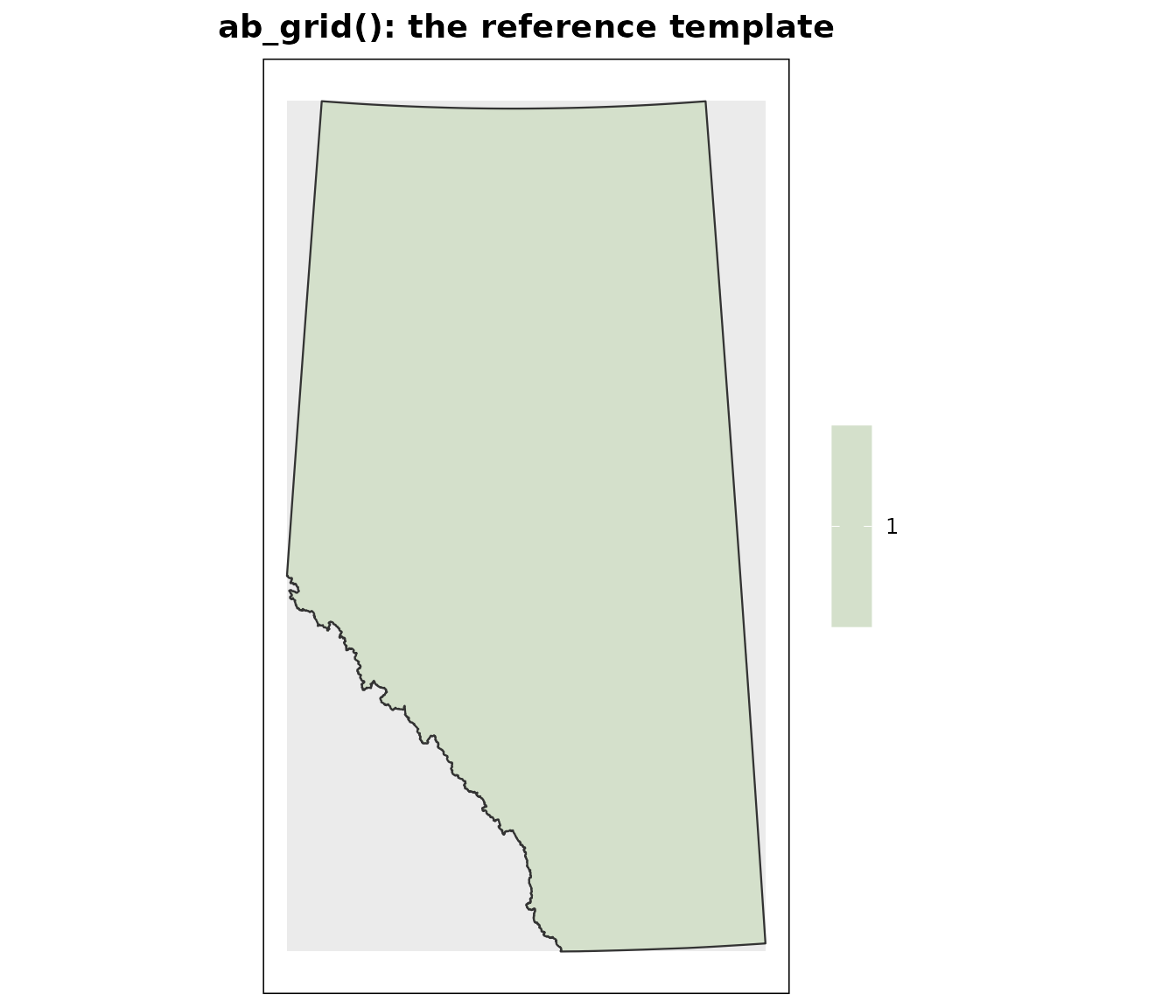
Cells covering Alberta hold 1; everything else is NA. Of the 857,630 cells in the rectangle, the province occupies:

global(ref, "notNA")
#>           notNA
#> grid_1km 664762

Colouring the NA cells shows the shape of that: a rectangle of 1 km cells, with values only where the province is.

plot_raster(
  ref,
  na_col = "grey92",
  main   = "ab_grid(): the reference template"
)

Two properties are worth knowing before you rely on it.

The template is *snapped to the lattice of the ABMI’s 1 km grid polygons (“\ABMI-DATA2_data1SQKM_AB2020_gdb”)*, not to a round number. That is why the origin is an odd pair of values rather than 0, 0:

origin(ref)
#> [1] -383.8178 -467.5689

The payoff is that a cell’s raster row and column reproduce its source GRID_LABEL, so raster work and the ABMI grid tabulations refer to the same cells.

Every raster cell is a full 1 km², whereas the source polygons along the provincial boundary are clipped to less than that. Area-weighted work on edge cells should go back to the source polygons on the share. Provenance for both layers is in inst/extdata/README.md.

ab_boundary()

The 2020 provincial boundary as one dissolved polygon, in the same CRS:

ab_boundary()
#> class       : SpatVector
#> geometry    : polygons
#> dimensions  : 1, 0  (geometries, attributes)
#> extent      : 170844.3, 865133.5, 5425575, 6659344  (xmin, xmax, ymin, ymax)
#> source      : alberta.gpkg
#> coord. ref. : NAD83 / Alberta 10-TM (Forest) (EPSG:3400)

It carries no attributes on purpose — it exists to clip, not to join to.

Checking alignment

check_alignment() compares a layer against the reference on all four properties and messages the result. The reference grid agrees with itself:

check_alignment(ref)
#> CRS: OK
#> Extent: OK
#> Resolution: OK
#> Origin: OK

Something freshly downloaded usually does not. Here is a stand-in for one — a synthetic temperature surface in geographic coordinates:

src <- rast(
  nrows = 120, ncols = 90,
  xmin = -121, xmax = -109,
  ymin = 48.5, ymax = 60.5,
  crs  = "EPSG:4326"
)
src <- 25 - 0.55 * init(src, "y") + 2 * sin(init(src, "x") / 2)
names(src) <- "mean_temp"
src
#> class       : SpatRaster
#> size        : 120, 90, 1  (nrow, ncol, nlyr)
#> resolution  : 0.1333333, 0.1  (x, y)
#> extent      : -121, -109, 48.5, 60.5  (xmin, xmax, ymin, ymax)
#> coord. ref. : lon/lat WGS 84 (EPSG:4326)
#> source(s)   : memory
#> name        :  mean_temp
#> min value   : -10.247308
#> max value   :    0.29701

It covers Alberta, on its own grid, in degrees. The provincial boundary is drawn on top for reference:

plot_raster(src, main = "As downloaded: EPSG:4326, ~0.1 degree")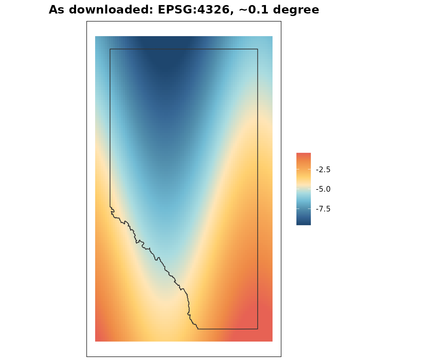

check_alignment(src)
#> CRS: MISMATCH — x and ref have different CRS.
#> Extent: MISMATCH.
#> Resolution: MISMATCH.
#> Origin: MISMATCH.

Four mismatches. The function can return the results invisibly as a named logical vector, so it can act as TRUE/FALSE gate in a code pipeline.

ok <- check_alignment(src, verbose = FALSE)
ok
#>        crs     extent resolution     origin 
#>      FALSE      FALSE      FALSE      FALSE
all(ok)
#> [1] FALSE

sf objects are accepted too, but only the CRS is meaningful for them. A point layer has no resolution or origin to compare, so those checks are skipped rather than silently reported as failures:

pts <- st_as_sf(
  data.frame(
    site = c("calgary", "edmonton"),
    x    = c(-114.07, -113.49),
    y    = c(51.05, 53.55)
  ),
  coords = c("x", "y"),
  crs    = 4326
)
check_alignment(pts)
#> CRS: MISMATCH — x and ref have different CRS.
#> Extent, resolution, and origin checks skipped (x is an sf object).

Get the CRS right first

This is a mandatory step. resample_to_grid() wraps terra::resample(), which aligns a layer to a template but does not reproject. Handed a layer in the wrong CRS it would treat the reference extent as though it were in the layer’s own coordinates, find nothing there, and return a raster of NA — a successful call producing an empty layer. resample_to_grid() refuses instead:

resample_to_grid(src)
#> Error:
#> ! CRS mismatch: `x` is WGS 84 and `ref` is NAD83 / Alberta 10-TM (Forest). resample_to_grid() does not reproject, and resampling across a CRS boundary returns an empty raster rather than an error. Reproject first:
#>   x <- terra::project(x, terra::crs(ref))

Reprojecting requires a separate call:

src_ab <- project(src, ab_crs())      # bilinear, fine for continuous
check_alignment(src_ab, verbose = FALSE)[["crs"]]
#> [1] TRUE

The CRS now agrees; the grid geometry still does not, which is what resample_to_grid() is for.

Harmonizing rasters

resample_to_grid()

With the CRS harmonized, resampling snaps the layer onto the reference lattice:

temp_1km <- resample_to_grid(src_ab)
#> resample_to_grid(): method = "bilinear" — continuous layer, refining (res 10,266 → 1,000, each input cell spans ~105 output cells); interpolating between input cell centres. Pass method = "near" to keep the values blocky.
temp_1km
#> class       : SpatRaster
#> size        : 1234, 695, 1  (nrow, ncol, nlyr)
#> resolution  : 1000, 1000  (x, y)
#> extent      : 170616.2, 865616.2, 5425532, 6659532  (xmin, xmax, ymin, ymax)
#> coord. ref. : NAD83 / Alberta 10-TM (Forest) (EPSG:3400)
#> source(s)   : memory
#> varname     : grid_1km
#> name        :  mean_temp
#> min value   : -10.046402
#> max value   :    0.10292
aligned <- check_alignment(temp_1km, verbose = FALSE)
aligned
#>        crs     extent resolution     origin 
#>       TRUE       TRUE       TRUE       TRUE

All four properties now agree, which is the whole point: any two layers put through this call can be stacked, differenced, or extracted from together.

plot_raster(temp_1km, main = "On the 1 km grid, still unclipped")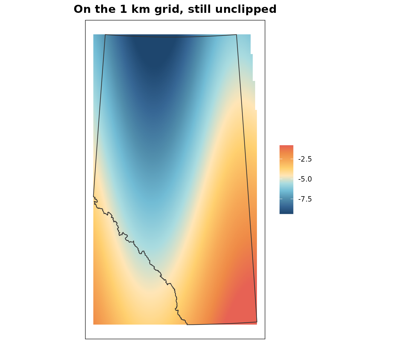

Same surface, now in metres on the reference lattice — and still carrying values well outside the province, which is what mask_to_boundary() is for.

Notice the output message:

#> resample_to_grid(): method = "bilinear" — continuous layer, refining (res 10,266 → 1,000, each input cell spans ~105 output cells); interpolating between input cell centres. Pass method = "near" to keep the values blocky.

terra::resample() always returns a layer on the reference geometry. What varies is how each output cell gets its value, and that is automatically determined based on the data type of the input raster and which way the resolution changes:

Direction	Continuous	Categorical
Coarsening (fine to coarse)	"average"	"mode"
Same resolution	"near"	"near"
Refining (coarse to fine)	"bilinear"	"near"

resample_to_grid() reads res(x) against res(ref), checks whether the layer is categorical, picks from that table, and says what it picked. Pass method to override it at any point.

Coarsening is the case that goes wrong quietly. A 30 m layer has roughly 1,111 cells inside every 1 km cell: "average" reads all of them, "bilinear" reads four, "near" reads one. All three produce a correctly aligned raster, and check_alignment() passes on all three, because alignment is about geometry and this is a question about values.

fine <- rast(
  xmin = 400000, xmax = 430000,
  ymin = 5800000, ymax = 5830000,
  res  = 30, crs = ab_crs()
)
set.seed(1)
values(fine) <- runif(ncell(fine), 0, 30)
win <- crop(ref, ext(400000, 430000, 5800000, 5830000))

by_mean <- resample_to_grid(fine, win)
#> resample_to_grid(): method = "average" — continuous layer, coarsening (res 30 → 1,000, ~1,111 input cells per output cell); averaging all of them.
by_near <- resample_to_grid(fine, win, method = "near")
#> resample_to_grid(): method = "near" (supplied).

# both align; they do not agree
all(check_alignment(by_near, win, verbose = FALSE))
#> [1] TRUE
mean(abs(values(by_mean) - values(by_near)), na.rm = TRUE)
#> [1] 7.293292
sd(values(by_mean), na.rm = TRUE)
#> [1] 0.2946164

Catagorical rasters: Interpolating between numerical land cover classes 1 and 3 defaults to "average" produces a 2, which is meaningless. Build a categorical layer from the same surface to see it:

zones <- classify(
  src,
  matrix(
    c(-Inf, -8, 1,
        -8, -5, 2,
        -5, -2, 3,
        -2, Inf, 4),
    ncol = 3, byrow = TRUE
  )
)
names(zones) <- "zone"
zones_ab <- project(zones, ab_crs(), method = "near")
sort(unique(values(zones_ab, na.rm = TRUE)))
#> [1] 1 2 3 4

A layer built this way holds class codes as plain numbers, so nothing marks it as categorical and resample_to_grid() automatically treats it as a continuous measurement:

wrong <- resample_to_grid(zones_ab, method = "bilinear")
#> resample_to_grid(): method = "bilinear" (supplied).
length(unique(values(wrong, na.rm = TRUE)))
#> [1] 26056
range(values(wrong, na.rm = TRUE))
#> [1] 1 4

Naming the method keeps them intact:

zone_1km <- resample_to_grid(zones_ab, method = "near")
#> resample_to_grid(): method = "near" (supplied).
sort(unique(values(zone_1km, na.rm = TRUE)))
#> [1] 1 2 3 4

Detection works off terra::is.factor(), so a layer with a proper level table is handled without being told:

zones_fct <- zones_ab
levels(zones_fct) <- data.frame(
  value = 1:4,
  zone  = c("cold", "cool", "mild", "warm")
)
auto_zone <- resample_to_grid(zones_fct)
#> resample_to_grid(): method = "near" — categorical layer, refining (res 10,266 → 1,000, each input cell spans ~105 output cells); nearest keeps the class codes intact.
sort(unique(values(auto_zone, na.rm = TRUE)))
#> [1] 1 2 3 4

Anything holding class codes as bare numbers needs method = given explicitly. That is the one thing the automatic choice cannot see.

Any resolution ratio

Summarising the fine cells using resample_to_grid() does not require the resolutions to divide evenly. terra::resample() works per output cell — each 1 km cell reads whatever falls inside it, 1,111 cells or 1,123 — rather than tiling the input into fixed blocks. A 300 m layer, which does not divide into 1 km at all, lands on the grid exactly:

odd <- rast(
  xmin = 400000, xmax = 430300,
  ymin = 5800000, ymax = 5830300,
  res  = 300, crs = ab_crs()
)
odd <- init(odd, "y")
res(odd)
#> [1] 300 300

odd_1km <- resample_to_grid(odd, win)
#> resample_to_grid(): method = "average" — continuous layer, coarsening (res 300 → 1,000, ~11 input cells per output cell); averaging all of them.
res(odd_1km)
#> [1] 1000 1000
all(check_alignment(odd_1km, win, verbose = FALSE))
#> [1] TRUE

Why terra::resample() and not terra::aggregate()? terra::aggregate() is more limited. Aggregation coarsens by an integer factor, and a factor is a single number: 1000 / 300 rounds to 3, giving 900 m cells. It also lays its blocks out from the input’s own corner, so it changes cell size without changing position.

Summaries beyond the mean

method accepts everything terra::resample() does, which covers most of what a coarse cell might need to say about the fine cells inside it:

totals <- resample_to_grid(fine, win, method = "sum")
#> resample_to_grid(): method = "sum" (supplied).
spread <- c(
  resample_to_grid(fine, win, method = "min"),
  resample_to_grid(fine, win, method = "max")
)
#> resample_to_grid(): method = "min" (supplied).
#> resample_to_grid(): method = "max" (supplied).
names(spread) <- c("min", "max")
global(spread, "mean", na.rm = TRUE)
#>            mean
#> min  0.02707072
#> max 29.97271530

"sum", "min", "q1", "median", "q3", "max", and "rms" are all available, alongside "average" and "mode".

For a summary not on that list — a standard deviation, an interquartile range, a function of your own — drop to terra::aggregate(), which takes an arbitrary function, then resample its output to snap it into place:

het <- aggregate(fine, fact = 33, fun = sd)   # 990 m, off-lattice
het_1km <- resample_to_grid(het, win)
#> resample_to_grid(): method = "average" — continuous layer, coarsening (res 990 → 1,000, ~1 input cell per output cell); averaging all of them.
all(check_alignment(het_1km, win, verbose = FALSE))
#> [1] TRUE

Two steps, and only because sd is not one of the built-in methods. For a mean, a mode, or a sum, one terra::resample() call does both jobs.

Output message

resample_to_grid() reports its choice of interpoloation method and the reason on every call. In a loop over a folder of covariates that log is the record of what happened to each layer, and it is where you can flag issues — a layer you thought was 1 km turning out to be 250 m, or a class raster being treated as continuous because its codes are stored as plain numbers. Pass quiet = TRUE to silence it.

The choice of method is a default, not a constraint. method overrides it whenever the layer’s meaning calls for something else — "sum" for counts, "near" for a layer whose exact values must survive, "bilinear" for a coarse smooth surface being refined.

mask_to_boundary()

Harmonizing to the grid gives a layer the right geometry but not the right footprint: a reprojected national product still carries values across almost the whole reference rectangle, including well outside Alberta.

global(temp_1km, "notNA")
#>            notNA
#> mean_temp 852260

Masking clips it to the province. The default boundary is "alberta", so the common call takes no second argument:

temp_ab <- mask_to_boundary(temp_1km)
global(temp_ab, "notNA")
#>            notNA
#> mean_temp 664749

plot_raster(temp_ab, main = "Clipped to Alberta")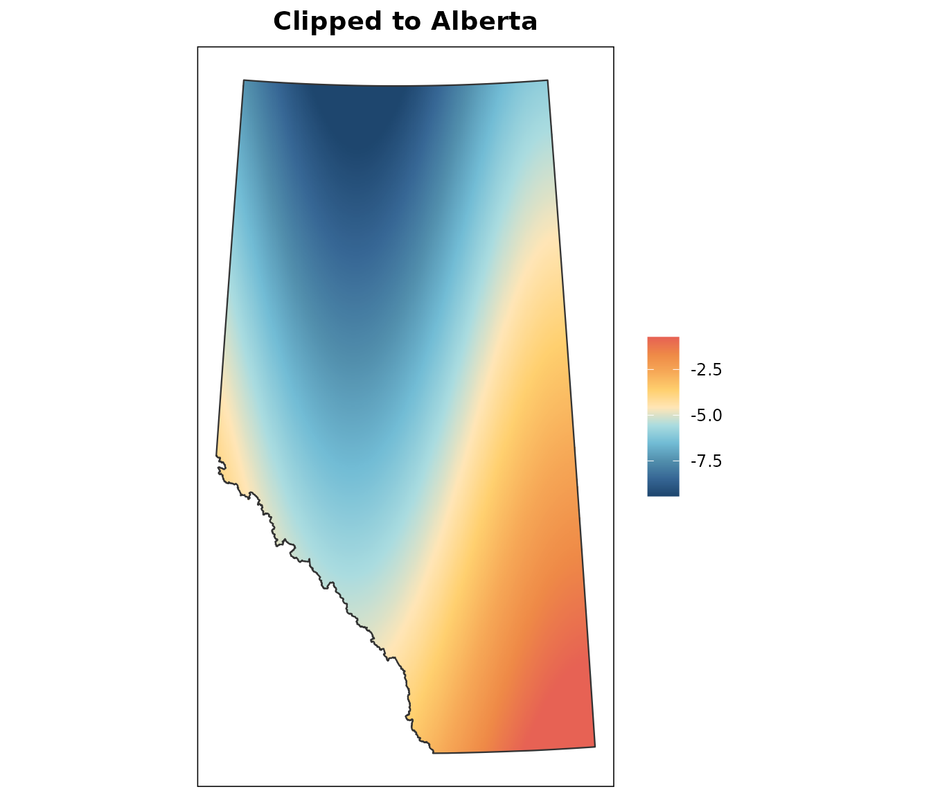

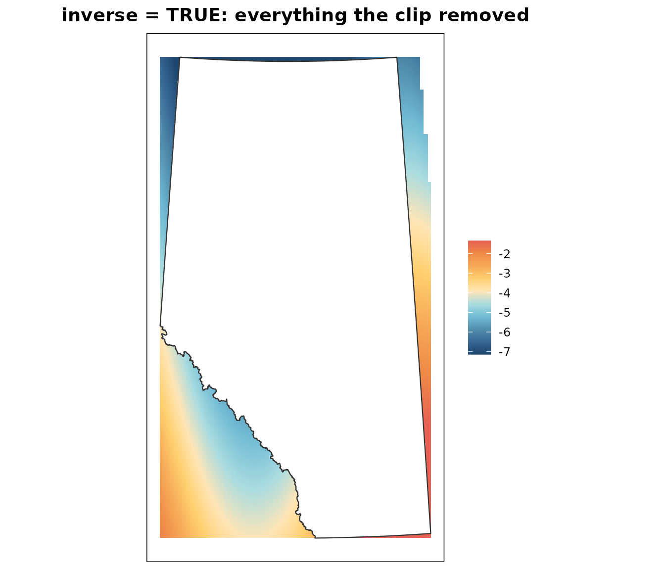
inverse = TRUE keeps the outside instead — useful for checking what a clip removed, or for building an outside-Alberta mask:

global(mask_to_boundary(temp_1km, inverse = TRUE), "notNA")
#>            notNA
#> mean_temp 187511

plot_raster(
  mask_to_boundary(temp_1km, inverse = TRUE),
  main = "inverse = TRUE: everything the clip removed"
)

Harmonizing points

Reprojecting points:

pts_ab <- harmonize_crs(pts)
#> Reprojecting `points` to the reference grid CRS (NAD83 / Alberta 10-TM (Forest)).
st_crs(pts_ab)$input
#> [1] "NAD83 / Alberta 10-TM (Forest)"
st_coordinates(pts_ab)
#>             X       Y
#> [1,] 565161.0 5653533
#> [2,] 600000.9 5932142

A worked pipeline

Everything above, as it would appear in a covariate-preparation script — a downloaded continuous layer and a point set, both brought onto the reference grid:

# 1. Check what arrived
check_alignment(src)
#> CRS: MISMATCH — x and ref have different CRS.
#> Extent: MISMATCH.
#> Resolution: MISMATCH.
#> Origin: MISMATCH.

# 2. CRS first; nothing else works until this passes
covariate <- project(src, ab_crs())

# 3. Snap to the reference grid
covariate <- resample_to_grid(covariate)
#> resample_to_grid(): method = "bilinear" — continuous layer, refining (res 10,266 → 1,000, each input cell spans ~105 output cells); interpolating between input cell centres. Pass method = "near" to keep the values blocky.

# 4. Clip to Alberta
covariate <- mask_to_boundary(covariate)

# 5. Confirm, do not assume
check_alignment(covariate)
#> CRS: OK
#> Extent: OK
#> Resolution: OK
#> Origin: OK

# 6. Bring the points into the same CRS
sites <- harmonize_crs(pts)
#> Reprojecting `points` to the reference grid CRS (NAD83 / Alberta 10-TM (Forest)).

covariate
#> class       : SpatRaster
#> size        : 1234, 695, 1  (nrow, ncol, nlyr)
#> resolution  : 1000, 1000  (x, y)
#> extent      : 170616.2, 865616.2, 5425532, 6659532  (xmin, xmax, ymin, ymax)
#> coord. ref. : NAD83 / Alberta 10-TM (Forest) (EPSG:3400)
#> source(s)   : memory
#> varname     : grid_1km
#> name        : mean_temp
#> min value   : -9.996937
#> max value   :  0.049084

From here extract_points() and the other extraction functions take over; they are covered separately.

Working off the default grid

Every reference default is an ordinary argument so defaults can be overridden for projects on a different grid or area of interest — a 250 m analysis, a single natural subregion, work outside Alberta.

own_ref <- rast(
  xmin = 400000, xmax = 500000,
  ymin = 5800000, ymax = 5900000,
  res  = 250, crs = ab_crs()
)
own <- resample_to_grid(src_ab, ref = own_ref)
#> resample_to_grid(): method = "bilinear" — continuous layer, refining (res 10,266 → 250, each input cell spans ~1,686 output cells); interpolating between input cell centres. Pass method = "near" to keep the values blocky.
all(check_alignment(own, ref = own_ref, verbose = FALSE))
#> [1] TRUE

ref is the argument for check_alignment() and resample_to_grid(); raster for harmonize_crs(); boundary for mask_to_boundary(). The package’s own reference layers are just the defaults those arguments carry, not a requirement.